Lesson 14 - Super Resolution; Image Segmentation with U-Net

These are my personal notes from fast.ai course and will continue to be updated and improved if I find anything useful and relevant while I continue to review the course to study much more in-depth. Thanks for reading and happy learning!

Topics

• Super resolution.
  • A technique that allows us to restore high resolution detail in our images, based on a convolutional neural network.
  • In the process, we'll look at a few modern techniques for faster and more reliable training of generative convnets.
• Image segmentation.
  • U-Net architecture.
    • A state of the art technique that has won many Kaggle competitions and is widely used in industry.
  • Image segmentation models allow us to precisely classify every part of an image, right down to pixel level.

Lesson Resources

• Website
• Video
• Wiki
• Jupyter Notebook and code
  • enhance.ipynb
  • style-transfer-net.ipynb
  • carvana.ipynb
  • carvana-unet.ipynb
• Dataset
  • ImageNet sample in files.fast.ai/data / direct download link (2.1 GB)
  • Full ImageNet [faster download from Kaggle, mirrored over from the ImageNet Download Site]
  • Kaggle Carvana Image Masking competition - you can download it with Kaggle API as usual

Assignments

Papers

• Must read
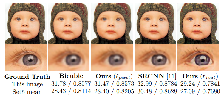
  • Perceptual Losses for Real-Time Style Transfer and Super-Resolution by Justin Johnson, et al.
  • Enhanced Deep Residual Networks for Single Image Super-Resolution (EDSR) by Bee Lim, et al.
  • Real-Time Single Image and Video Super-Resolution Using an Efficient Sub-Pixel Convolutional Neural Network by Wenzhe Shi, et al.
  • Checkerboard artifact free sub-pixel convolution: A note on sub-pixel convolution, resize convolution and convolution resize by Andrew Aitken, et al.
  • U-Net: Convolutional Networks for Biomedical Image Segmentation by Olaf Ronneberger, et al.
• Additional papers (optional)
  • Feature Pyramid Networks for Object Detection by Tsung-Yi Lin, Piotr Dollar, Ross Girshick, Kaiming He, et al.

My Notes

Show and tell from last week

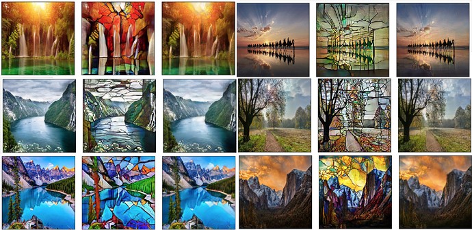
Alena Harley did something really interesting which was she tried finding out what would happen if you did CycleGAN on just three or four hundred images and I really like these projects where people just go to Google Image Search using the API or one of the libraries out there. Some of our students have created some very good libraries for interacting with Google images API to download a bunch of stuff they are interested in, in this case some photos and some stained glass windows. With 300~400 photos of that, she trained a few different model — this is what I particularly liked. As you can see, with quite a small number of images, she gets very nice stained-glass effects. So I thought that was an interesting example of using pretty small amounts of data that was readily available that she was able to download pretty quickly. There is more information about that on the forum if you are interested. It's interesting to wonder about what kinds of things people will come up with with this kind of generative model. It's clearly a great artistic medium. It's clearly a great medium for forgeries and fakeries. I wonder what other kinds of things people will realize they can do with these kind of generative models. I think audio is going to be the next big area. Also very interactive type stuff. Nvidia just released a paper showing an interactive kind of photo repair tool where you just brush over an object and it replaces it with a deep learning generated replacement very nicely. Those kinds of interactive tools, I think would be very interesting too.

Super Resolution [00:02:06]

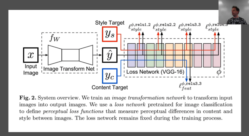
Perceptual Losses for Real-Time Style Transfer and Super-Resolution paper

Last time, we looked at doing style transfer by actually directly optimizing pixels. Like with most of the things in part two, it's not so much that I'm wanting you to understand style transfer per se, but the kind of idea of optimizing your input directly and using activations as part of a loss function is really the key takeaway here.

So it's interesting then to see effectively the follow-up paper, not from the same people but the paper that came next in the sequence of these vision generative models with this one from Justin Johnson and folks at Stanford. It actually does the same thing — style transfer, but does it in a different way. Rather than optimizing the pixels, we are going to go back to something much more familiar and optimize some weights. So specifically, we are going to train a model which learns to take a photo and translate it into a photo on this in the style of a particular artwork. So each conv net will learn to produce one kind of style.

Now it turns out that getting to that point, there is an intermediate point which (I actually think more useful and takes us half way there) is something called super resolution. So we are actually going to start with super resolution [00:03:55]. Because then we'll build on top of super resolution to finish off the conv net based style transfer.

Super resolution is where we take a low resolution image (we are going to take 72 by 72) and upscale it to a larger image (288 by 288 in our case) trying to create a higher res image that looks as real as possible. This is a challenging thing to do because at 72 by 72, there's not that much information about a lot of the details. The cool thing is that we are going to do it in a way as we tend to do with vision models which is not tied to the input size so you could totally then take this model and apply it to a 288 by 288 image and get something that's four times bigger on each side so 16 times bigger than the original. Often it even works better at that level because you're really introducing a lot of detail into the finer details and you could really print out a high resolution print of something which earlier on was pretty pixelated.

Notebook: enhance.ipynb [00:05:06]

It is a lot like that kind of CSI style enhancement where we're going to take something that appears like the information is just not there and we kind of invent it — but the conv net is going to learn to invent it in a way that's consistent with the information that is there, so hopefully it's inventing the right information. One of the really nice things about this kind of problem is that we can create our own dataset as big as we like without any labeling requirements because we can easily create a low res image from a high res image just by down sampling our images. 🔖 So something I would love some of you to try this week would be to do other types of image-to-image translation where you can invent "labels" (your dependent variables). For example:

• Deskewing: Either recognize things that have been rotated by 90 degrees or better still that have been rotated by 5 degrees and straighten them.
• Colorization: Make a bunch of images into black-and-white and learn to put the color back again.
• Noise-reduction: Maybe do a really low quality JPEG save, and learn to put it back to how it should have been.
• Maybe taking something that's in a 16 color palette and put it back to a higher color palette.

I think these things are all interesting because they can be used to take pictures that you may have taken back on crappy old digital cameras before there are high resolution or you may have scanned in some old photos that are now faded, etc. I think it's really useful thing to be able to do and it's a good project because it's really similar to what we are doing here but different enough that you come across some interesting challenges on the way, I'm sure.

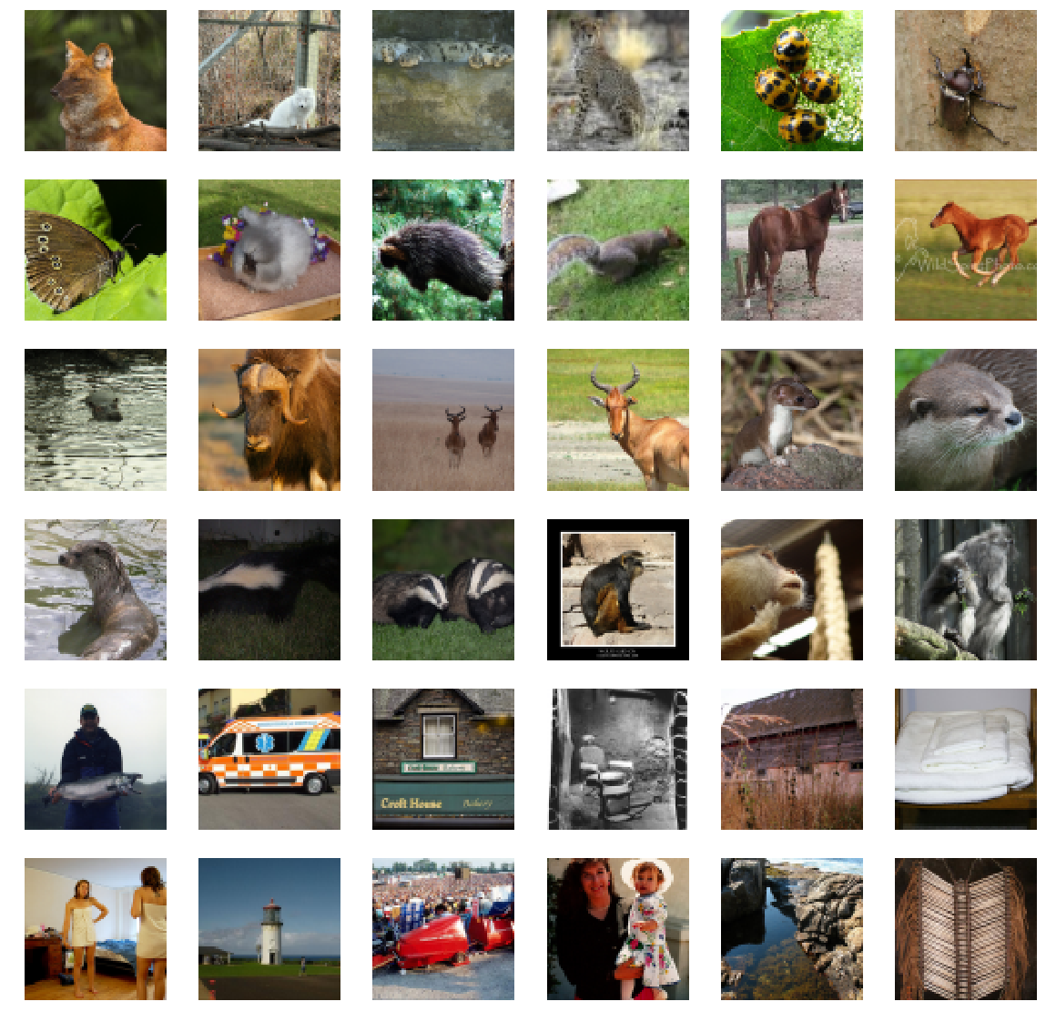
I'm going to use ImageNet again [00:07:19]. You don't need to use all of the ImageNet at all, I just happen to have it lying around. You can download the one percent sample of ImageNet from files.fast.ai. You can use any set of pictures you have lying around honestly.

matplotlib inline
%reload_ext autoreload
%autoreload 2

Super resolution data

from fastai.conv_learner import *
from pathlib import Path
# torch.cuda.set_device(0)

torch.backends.cudnn.benchmark = True

PATH = Path('data/imagenet')
PATH_TRN = PATH / 'train'

In this case, as I say we don't really have labels per se, so I'm just going to give everything a label of zero just so we can use it with our existing infrastructure more easily.

fnames_full, label_arr_full, all_labels = folder_source(PATH, 'train')
fnames_full = ['/'.join(Path(fn).parts[-2:]) for fn in fnames_full]
list(zip(fnames_full[:5], label_arr_full[:5]))

# -----------------------------------------------------------------------------
# Output
# -----------------------------------------------------------------------------
[('n01440764/n01440764_12241.JPEG', 0),
 ('n01440764/n01440764_529.JPEG', 0),
 ('n01440764/n01440764_11155.JPEG', 0),
 ('n01440764/n01440764_9649.JPEG', 0),
 ('n01440764/n01440764_8013.JPEG', 0)]

all_labels[:5]

# -----------------------------------------------------------------------------
# Output
# -----------------------------------------------------------------------------
['n01440764', 'n01443537', 'n01491361', 'n01494475', 'n01498041']

Now, because I'm pointing at a folder that contains all of ImageNet, I certainly don't want to wait for all of ImageNet to finish to run an epoch. So here, I'm just, most of the time, I would set "keep percent" (keep_pct) to 1 or 2%. And then I just generate a bunch of random numbers and then I just keep those which are less than 0.02 and so that lets me quickly subsample my rows.

np.random.seed(42)
keep_pct = 1.
# keep_pct = 0.02
keeps = np.random.rand(len(fnames_full)) < keep_pct
fnames = np.array(fnames_full, copy=False)[keeps]
label_arr = np.array(label_arr_full, copy=False)[keeps]

Architecture

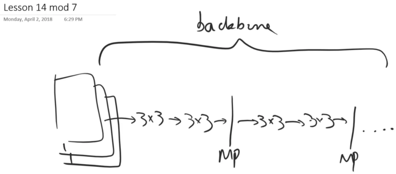
So we are going to use VGG16 [00:08:21] and VGG16 is something that we haven't really looked at in this class but it's a very simple model where we take our normal presumably 3 channel input, and we basically run it through a number of 3x3 convolutions, and then from time to time, we put it through a 2x2 maxpool and then we do a few more 3x3 convolutions, maxpool, so on so forth. And this is our backbone.

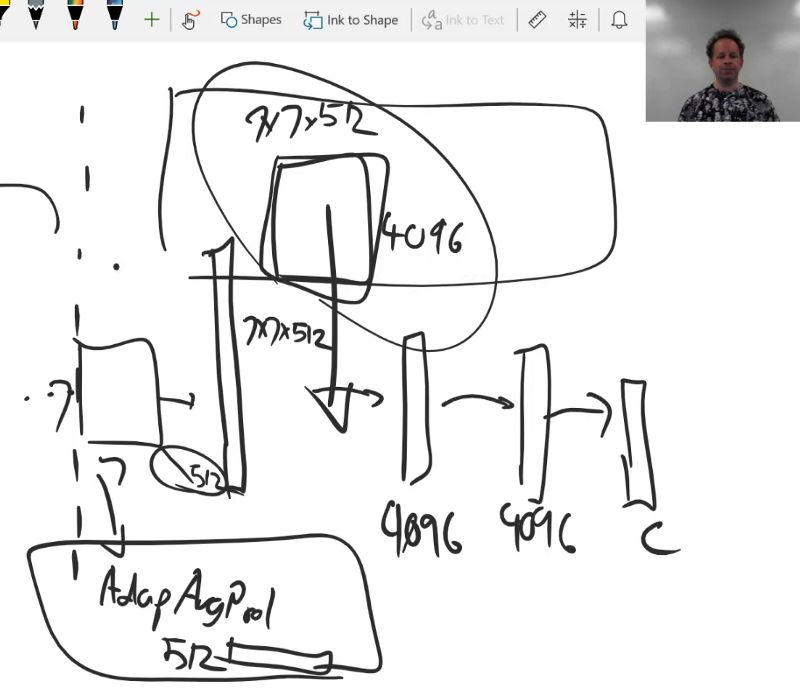
Then we don't do an adaptive average pooling layer. After a few of these, we end up with this 7x7x512 grid as usual (or something similar). So rather than average pooling, we do something different which is we flatten the whole thing — so that spits out a very long vector of activations of size 7x7x512 if memory serves correctly. Then that gets fed into two fully connected layers each one of which has 4096 activations, and one more fully connected layer which has however many classes. So if you think about it, the weight matrix here, it's HUGE 7x7x512x4096. It's because of that weight matrix really that VGG went out of favor pretty quickly — because it takes a lot of memory and takes a lot of computation and it's really slow. And there's a lot of redundant stuff going on here because really those 512 activations are not that specific to which of those 7x7 grid cells they are in. But when you have this entire weight matrix here of every possible combination, it treats all of them uniquely. So that can also lead to generalization problems because there's just a lot of weights and so forth.

Modern network approach

My view is that the approach that is used in every modern network which is here we do an adaptive average pooling (in Keras it's known as a global average pooling, in fast.ai, we do an AdaptiveConcatPool) which spits it straight down to a 512 long activation [00:11:06]. I think that's throwing away too much geometry. 🔖 So to me, probably the correct answer is somewhere in between and will involve some kind of factored convolution or some kind tensor decomposition which maybe some of us can think about in the coming months. So for now, anyway, we've gone from one extreme which is the adaptive average pooling to the other extreme which is this huge flattened fully connected layer.

Create something that's good at a lots of things

A couple of things which are interesting about VGG that make it still useful today [00:11:59]. The first one is that there's more interesting layers going on here with most modern networks including the ResNet family, the very first layer generally is a 7x7 conv with stride 2 or something similar. Which means we throw away half the grid size straight away and so there is little opportunity to use the fine detail because we never do any computation with it. So that's a bit of a problem for things like segmentation or super resolution models because the fine details matters. We actually want to restore it. Then the second problem is that the adaptive pooling layer entirely throws away the geometry in the last few sections which means that the rest of the model doesn't really have as much interesting kind of learning that geometry as it otherwise might. Therefore for things which are dependent on position, any kind of localization based approach to anything that requires generative model is going to be less effective. So one of the things I'm hoping you are hearing as I describe this is that probably none of the existing architectures are actually ideal. We can invent a new one. Actually, I just tried inventing a new one over the week which was to take the VGG head and attach it to a ResNet backbone. Interestingly, I found I actually got a slightly better classifier than a normal ResNet but it also was something with a little bit more useful information in it. It took 5 or 10% longer to train but nothing worth worrying about. Maybe we could, in ResNet, replace this (7x7 conv stride 2) as we've talked about briefly before. This very early convolution with something more like an Inception stem which has a bit more computation. I think there's definitely room for some nice little tweaks to these architectures so that we can build some models which are maybe more versatile. At the moment, people tend to build architectures that just do one thing. They don't really think what am I throwing away in terms of opportunity because that's how publishing works. You published "I've got state of the art of this one thing rather than you have created something that's good at a lots of things.

For these reasons, we are going to use VGG today even though it's ancient and it's missing lots of great stuff [00:14:42]. One thing we are going to do though is use a slightly more modern version which is a version of VGG where batch norm has been added after all the convolutions. In fast.ai when you ask for a VGG network, you always get the batch norm one because that's basically always what you want. So this is VGG with batch norm. There is 16 and 19, the 19 is way bigger and heavier, and doesn't really do any better, so no one really uses it.

arch = vgg16
sz_lr = 72

We are going to go from 72 by 72 LR (sz_lr: size low resolution) input. We are going to initially scale it up by times 2 with the batch size of 64 to get 2 * 72 so 144 by 144 output. That is going to be our stage one.

scale, bs = 2, 64
# scale, bs = 4, 32
sz_hr = sz_lr * scale

We'll create our own dataset for this and it's very worthwhile looking inside the fastai.dataset module and seeing what's there [00:15:45]. Because just about anything you'd want, we probably have something that's almost what you want. So in this case, I want a dataset where my x's are images and my y's are also images. There's already a files dataset we can inherit from where the x's are images and then I just inherit from that and I just copied and pasted the get_x and turn that into get_y so it just opens an image. Now I've got something where the x is an image and the y is an image, and in both cases, what we're passing in is an array of files names.

class MatchedFilesDataset(FilesDataset):
    def __init__(self, fnames, y, transforms, path):
        self.y = y
        assert(len(fnames) == len(y))
        super().__init__(fnames, transform, path)

    def get_y(self, i): return open_image(os.path.join(self.path, self.y[i]))

    def get_c(self): return 0

I'm going to do some data augmentation [00:16:32]. Obviously with all of ImageNet, we don't really need it but this is mainly here for anybody who is using smaller datasets to make the most of it. RandomDihedral is referring to every possible 90 degree rotation plus optional left/right flipping so they are dihedral group of eight symmetries. Normally we don't use this transformation for ImageNet pictures because you don't normally flip dogs upside down but in this case, we are not trying to classify whether it's a dog or a cat, we are just trying to keep the general structure of it. So actually every possible flip is a reasonably sensible thing to do for this problem.

aug_tfms = [RandomDihedral(tfm_y=TfmType.PIXEL)]

Create a validation set in the usual way [00:17:19]. You can see I'm using a few more slightly lower level functions — generally speaking, I just copy and paste them out of the fastai source code to find the bits I want. So here is the bit which takes an array of validation set indexes and one or more arrays of variables, and simply splits. In this case, this (np.array(fnames)) into a training and validation set, and this (the second np.array(fnames)) into a training and validation set to give us our x's and our y's. In this case, the x and the y are the same. Our input image and our output image are the same. We are going to use transformations to make one of them lower resolution. That's why these are the same thing.

val_idxs = get_cv_idxs(len(fnames), val_pct=min(0.01 / keep_pct, 0.1))
((val_x, trn_x), (val_y, trn_y)) = split_by_idx(val_idxs, np.array(fnames), np.array(fnames))
len(val_x), len(trn_x)

# -----------------------------------------------------------------------------
# Output
# -----------------------------------------------------------------------------
(194, 19245)

img_fn = PATH / 'train' / 'n01558993' / 'n01558993_9684.JPEG'

The next thing that we need to do is to create our transformations as per usual [00:18:13]. We are going to use tfm_y parameter like we did for bounding boxes but rather than use TfmType.COORD we are going to use TfmType.PIXEL. That tells our transformations framework that your y values are images with normal pixels in them, so anything you do to the x, you also need to do the same thing to the y. You need to make sure any data augmentation transformations you use have the same parameter as well.

tfms = tfms_from_model(arch, sz_lr, tfm_y=TfmType.PIXEL, aug_tfms=aug_tfms, sz_y=sz_hr)
datasets = ImageData.get_ds(MatchedFilesDataset, (trn_x, trn_y), (val_x, val_y), tfms, path=PATH_TRN)
md = ImageData(PATH, datasets, bs, num_workers=16, classes=None)

You can see the possible transform types you got:

• CLASS: classification which we are about to use the segmentation in the second half of today
• COORD: coordinates — no transformation at all
• PIXEL

Once we have Dataset class and some x and y training and validation sets. There is a handy little method called get datasets (get_ds) which basically runs that constructor over all the different things that you have to return all the datasets you need in exactly the right format to pass to a ModelData constructor (in this case the ImageData constructor). So we are kind of going back under the covers of fastai a little bit and building it up from scratch. In the next few weeks, this will all be wrapped up and refactored into something that you can do in a single step in fastai. But the point of this class is to learn a bit about going under the covers.

Something we've briefly seen before is that when we take images in, we transform them not just with data augmentation but we also move the channel dimension up to the start, we subtract the mean divided by the standard deviation etc [00:20:08]. So if we want to be able to display those pictures that have come out of our datasets or data loaders, we need to de-normalize them. So the model data object's (md) dataset (val_ds) has denorm function that knows how to do that. I'm just going to give that a short name for convenience:

denorm = md.val_ds.denorm

So now I'm going to create a function that can show an image from a dataset and if you pass in something saying this is a normalized image, then we'll denorm it.

def show_img(ims, idx, figsize=(5,5), normed=True, ax=None):
    if ax is None:
        fig, ax = plt.subplots(figsize=figsize)
    if normed:
        ims = denorm(ims)
    else:
        ims = np.rollaxis(to_np(ims), 1, 4)
    ax.imshow(np.clip(ims, 0, 1)[idx])
    ax.axis('off')

x, y = next(iter(md.val_dl))
x.size(), y.size()

# -----------------------------------------------------------------------------
# Output
# -----------------------------------------------------------------------------
(torch.Size([64, 3, 72, 72]), torch.Size([64, 3, 144, 144]))

You'll see here we've passed in size low res (sz_lr) as our size for the transforms and size high res (sz_hr) as, this is something new, the size y parameter (sz_y) [00:20:58]. So the two bits are going to get different sizes.

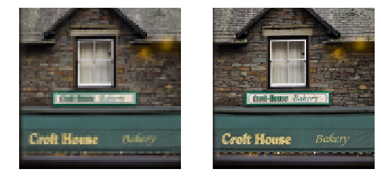
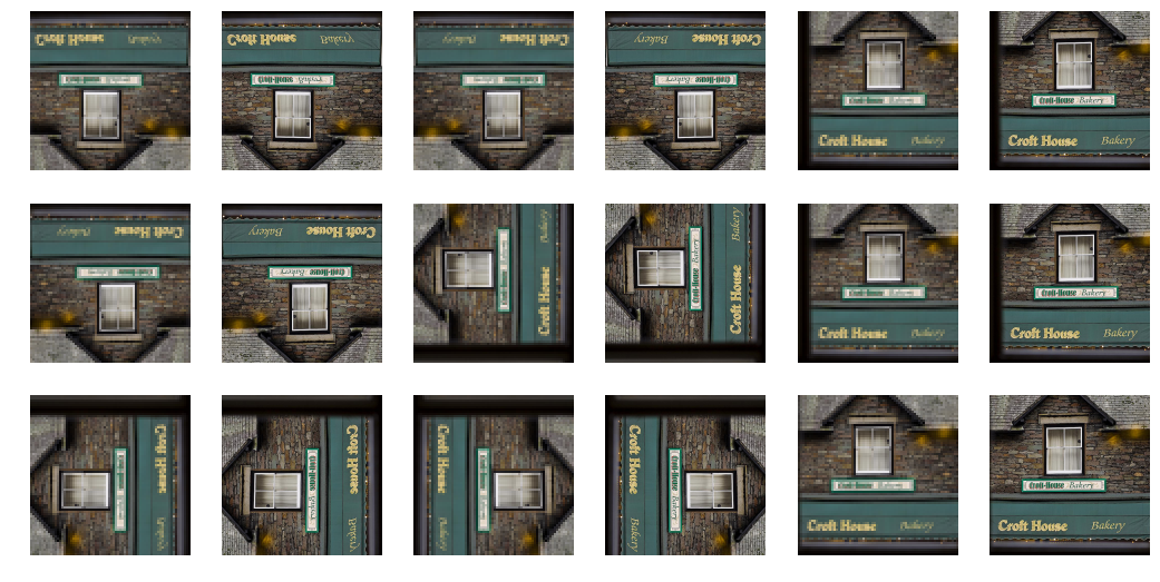
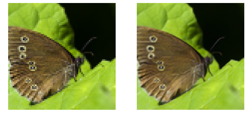
Here you can see the two different resolutions of our x and our y for a whole bunch of bakery.

idx = 61
fig, axes = plt.subplots(1, 2, figsize=(9, 5))
show_img(x, idx, ax=axes[0])
show_img(y, idx, ax=axes[1])

As per usual, plt.subplots to create our two plots and then we can just use the different axes that came back to put stuff next to each other.

batches = [next(iter(md.aug_dl)) for i in range(9)]

We can then have a look at a few different versions of the data transformation [00:21:37]. There you can see them being flipped in all different directions.

fig, axes = plt.subplots(3, 6, figsize=(18, 9))

for i,(x, y) in enumerate(batches):
    show_img(x, idx, ax=axes.flat[i*2])
    show_img(y, idx, ax=axes.flat[i*2+1])

Model [00:21:48]

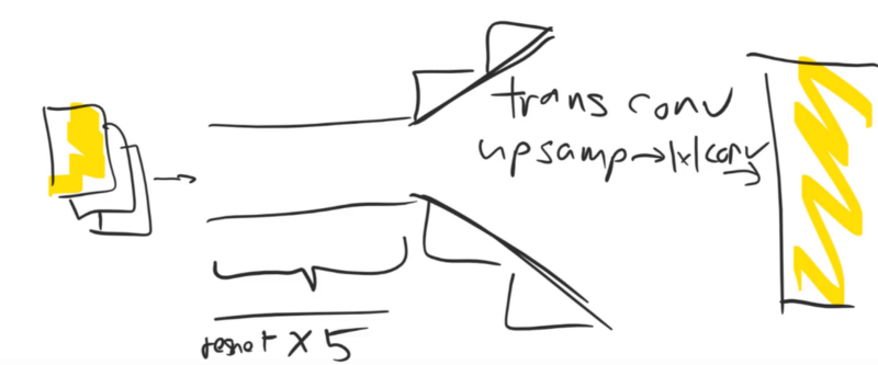
Let's create our model. We are going to have a small image coming in, and we want to have a big image coming out. So we need to do some computation between those two to calculate what the big image would look like. Essentially there're two ways of doing that computation:

• We could first of all do some upsampling and then do a few stride one layers to do lots of computation.
• We could first do lots of stride one layers to do all the computation and then at the end do some upsampling.

We are going to pick the second approach because we want to do lots of computation on something smaller because it's much faster to do it that way. Also, all that computation we get to leverage during the upsampling process. Upsampling, we know a couple of possible ways to do that. We can use:

• Transposed or fractionally strided convolutions
• Nearest neighbor upsampling followed by a 1x1 conv

And in "do lots of computation" section, we could just have a whole bunch of 3x3 convs. But in this case particular, it seems likely that ResNet blocks are going to be better because really the output and the input are very very similar. So we really want a flow through path that allows as little fussing around as possible except a minimal amount necessary to do our super resolution. If we use ResNet blocks, then they have an identity path already. So you can imagine those simple version where it does a bilinear sampling approach or something it could just go through identity block all the way through and then in the upsampling blocks, just learn to take the averages of the inputs and get something that's not too terrible.

So that's what we are going to do. We are going to create something with five ResNet blocks and then for each 2x scale up we have to do, we'll have one upsampling block.

They are all going to consist of, as per usual, convolution layers possibly with activation functions after many of them [00:24:37]. I like to put my standard convolution block into a function so I can refactor it more easily. I won't worry about passing in padding and just calculate it directly as kernel size over two.

def conv(ni, nf, kernel_size=3, actn=False):
    """Standard convolution block"""
    layers = [nn.Conv2d(ni, nf, kernel_size, padding=kernel_size//2)]
    if actn:
        layers.append(nn.ReLU(True))
    return nn.Sequential(*layers)

EDSR idea

One interesting thing about our little conv block is that there is no batch norm which is pretty unusual for ResNet type models.

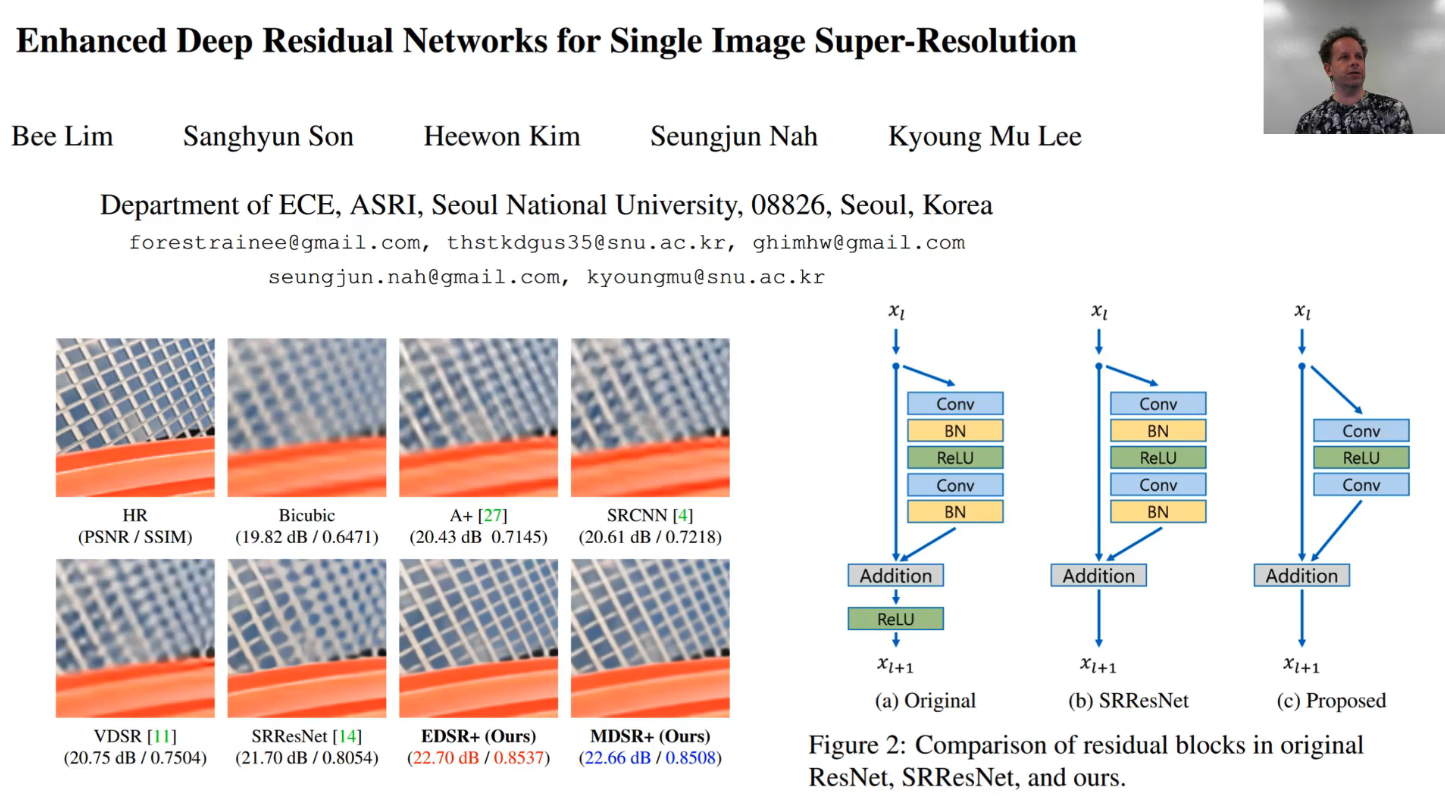
The reason there is no batch norm is because I'm stealing ideas from this fantastic recent paper which actually won a recent competition in super resolution performance. To see how good this paper is, SRResNet is the previous state of the art and what they've done here is they've zoomed way in to an upsampled mesh/fence. HR is the original. You can see in the previous best approach, there's a whole lot of distortion and blurring going on. Or else, in their approach, it's nearly perfect. So this paper was a really big step-up. They call their model EDSR (Enhanced Deep Super-Resolution network) and they did two things differently to the previous standard approaches:

1. Take the ResNet blocks and throw away the batch norms. Why would they throw away the batch norm? The reason is because batch norm changes stuff and we want a nice straight through path that doesn't change stuff. So the idea here is if you don't want to fiddle with the input more than you have to, then don't force it to have to calculate things like batch norm parameters — so throw away the batch norm.
2. Scaling factor (we will see shortly).

class ResSequential(nn.Module):
    def __init__(self, layers, res_scale=1.0):
        super().__init__()
        self.res_scale = res_scale
        self.m = nn.Sequential(*layers)

    def forward(self, x):
        return x + self.m(x) * self.res_scale

So we are going to create a residual block containing two convolutions. As you see in their approach, they don't even have a ReLU after their second conv. So that's why I've only got activation on the first one.

def res_block(nf):
    return ResSequential(
        [conv(nf, nf, actn=True), conv(nf, nf)],
        0.1)

A couple of interesting things here [00:27:10]. One is that this idea of having some kind of a main ResNet path (conv, ReLU, conv) and then turning that into a ReLU block by adding it back to the identity — it's something we do so often that I factored it out into a tiny little module called ResSequential. It simply takes a bunch of layers that you want to put into your residual path, turns that into a sequential model, runs it, and then adds it back to the input. With this little module, we can now turn anything, like conv activation conv, into a ResNet block just by wrapping in ResSequential.

Batch normalization

But that's not quite all I'm doing because normally a Res block just has x + self.m(x) in its forward. But I've also got * self.res_scale. What's res_scale? res_scale is the number 0.1. Why is it there? I'm not sure anybody quite knows. But the short answer is that the guy (Christian Szegedy) who invented batch norm also somewhat more recently did a paper in which he showed for (I think) the first time the ability to train ImageNet in under an hour. The way he did it was fire up lots and lots of machines and have them work in parallel to create really large batch sizes. Now generally when you increase the batch size by order N, you also increase the learning rate by order N to go with it. So generally a very large batch size training means very high learning rate training as well. He found that with these very large batch sizes of 8,000+ or even up to 32,000, at the start of training, his activations would basicall go straight to infinity. And a lot of other people have found that. We actually found that when we were competing in DAWNBench both on the CIFAR10 and ImageNet competitions that we really struggled to make the most of even the eight GPUs that we were trying to take advantage of because of these challenges with these larger batch sizes and taking advantage of them. Something Christian found was that in the ResNet blocks, if he multiplied them by some number smaller than 1, something like .1 or .2, it really helped stabilize training at the start. That's kind of weird because mathematically, it's identical. Because obviously whatever I'm multiplying it by here, I could just scale the weights by the opposite amount and have the same number. But we are not dealing with abstract math — we are dealing with real optimization problems, different initializations, learning rates, and whatever else. So the problem of weights disappearing off into infinity, I guess generally is really about the discrete and finite nature of computers in practice partly. So often these kind of little tricks can make the difference.

In this case, we are just toning things down based on our initial initialization. So there are probably other ways to do this. For example, one approach from some folks at Nvidia called LARS which I briefly mentioned last week is an approach which uses discriminative learning rates calculated in real time. Basically looking at the ratio between the gradients and the activations to scale learning rates by layer. So they found that they didn't need this trick to scale up the batch sizes a lot. Maybe a different initialization would be all that's necessary. The reason I mentioned this is not so much because I think a lot of you are likely to want to train on massive clusters of computers but rather that I think a lot of you want to train models quickly and that means using high learning rates and ideally getting super convergence. I think these kinds of tricks are the tricks that we'll need to be able to get super convergence across more different architectures and so forth. Other than Leslie Smith, no one else is really working on super convergence other than some fastai students nowadays. So these kind of things about how do we train at very very high learning rates, we're going to have to be the ones who figure it out because as far as I can tell, nobody else cares yet. So looking at the literature around training ImageNet in one hour, or more recently there's now train ImageNet in 15 minutes, these papers actually, I think, have some of the tricks to allow us to train things at high learning rates. So here is one of them.

Interestingly, other than the train ImageNet in one hour paper, the only other place I've seen this mentioned was in this EDSR paper. It's really cool because people who win competitions, I find them to be very pragmatic and well-read. They actually have to get things to work. So this paper describes an approach which actually worked better than anybody else's approach and they did these pragmatic things like throw away batch norm and use this little scaling factor which almost nobody seems to know about. So that's where .1 comes from.

def upsample(ni, nf, scale):
    layers = []
    for i in range(int(math.log(scale, 2))):
        layers += [conv(ni, nf*4), nn.PixelShuffle(2)]
    return nn.Sequential(*layers)

So basically our super-resolution ResNet (SrResnet) is going to do a convolution to go from our three channels to 64 channels just to richen up the space a little bit [00:33:25]. Then also we've got actually 8 not 5 Res blocks. Remember, every one of these Res block is stride 1 so the grid size doesn't change, the number of filters doesn't change. It's just 64 all the way through. We'll do one more convolution, and then we'll do our upsampling by however much scale we asked for. Then something I've added which is one batch norm here because it felt like it might be helpful just to scale the last layer. Then finally conv to go back to the three channels we want. So you can see that here's lots and lots of computation and then a little bit of upsampling just like we described.

class SrResnet(nn.Module):
    def __init__(self, nf, scale):
        super().__init__()
        features = [conv(3, 64)]

        for i in range(8):
            features.append(res_block(64))

        features += [
            conv(64, 64),
            upsample(64, 64, scale),
            nn.BatchNorm2d(64),
            conv(64, 3)
        ]
        self.features = nn.Sequential(*features)

    def forward(self, x):
        return self.features(x)

Just to mention, as I'm tending to do now, this whole thing is done by creating a list with layers and then at the end, turning into a sequential model so my forward function is as simple as can be.

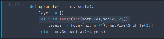
Here is our upsampling and upsampling is a bit interesting because it is not doing either of two things (transposed or fractionally strided convolutions or nearest neighbor upsampling followed by a 1x1 conv). So let's talk a bit about upsampling.

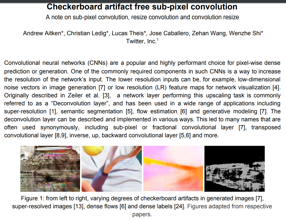
Here is the picture from the paper (Perceptual Losses for Real-Time Style Transfer and Super Resolution). So they are saying "hey, our approach is so much better" but look at their approach. It's got artifacts in it. These just pop up everywhere, don't they. One of the reason for this is that they use transposed convolutions and we all know, don't use transposed convolutions.

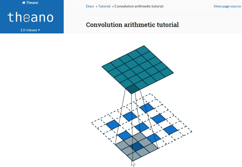
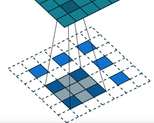
Here are transposed convolutions [00:35:39]. This is from this fantastic convolutional arithmetic paper that was shown also in the Theano docs. If we are going from (blue is the original image) 3x3 image up to a 5x5 image (6x6 if we added a layer of padding), then all a transpose convolution does is it uses a regular 3x3 conv but it sticks white zero pixels between every pair of pixels. That makes the input image bigger and when we run this convolution over it, therefore gives us a larger output. But that's obviously stupid because when we get here, for example, of the nine pixels coming in, eight of them are zero. So we are just wasting a whole a lot of computation. On the other hand, if we are slightly off then four of our nine are non-zero. But yet, we only have one filter/kernel to use so it can't change depending on how many zeros are coming in. So it has to be suitable for both and it's just not possible so we end up with these artifacts.

One approach we've learnt to make it a bit better is to not put white things here but instead to copy the pixel's value to each of these three locations [00:36:53]. So that's a nearest neighbor upsampling. That's certainly a bit better, but it's still pretty crappy because now when we get to these nine (as shown above), 4 of them are exactly the same number. And when we move across one, then now we've got a different situation entirely. So depending on where we are, in particular, if we are here, there's going to be a lot less repetition:

So again, we have this problem where there's wasted computation and too much structure in the data, and it's going to lead to artifacts again. So upsampling is better than transposed convolutions — it's better to copy them rather than replace them with zero. But it's still not quite good enough.

Pixel shuffle

So instead, we are going to do the pixel shuffle [00:37:56]. Pixel shuffle is an operation in this sub-pixel convolutional neural network and it's a little bit mind-bending but it's kind of fascinating.

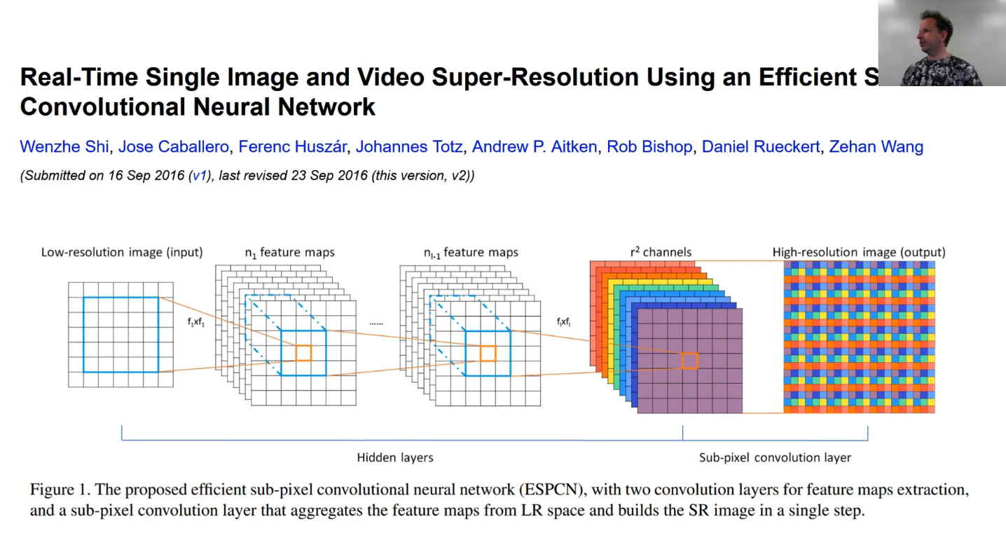
We start with our input, we go through some convolutions to create some feature maps for a while until eventually we get to layer n[i-1] which has n[i-1] feature maps. We are going to do another 3x3 conv and our goal here is to go from a 7x7 grid cell (we're going to do a 3x3 upscaling) so we are going to go up to a 21x21 grid cell. So what's another way we could do that? To make it simpler, let's just pick one face/layer- so let's take the top most filter and just do a convolution over that just to see what happens. What we are going to do is we are going to use a convolution where the kernel size (the number of filters) is nine times bigger than we need (strictly speaking). So if we needed 64 filters, we are actually going to do 64 times 9 filters. Why? Here, r is the scale factor so 3² is 9, so here are the nine filters to cover one of these input layers/slices. But what we can do is we started with 7x7, and we turned it into 7x7x9. The output that we want is equal to 7 times 3 by 7 times 3. In other words, there is an equal number of pixels/activations here as there are activations in the previous step. So we can literally re-shuffle these 7x7x9 activations to create this 7x3 by 7x3 map [00:40:16]. So what we are going to do is we're going to take one little tube here (all the top left hand of each grid) and we are going to put the purple one up in the top left, then the blue one one to the right, and light blue one on to the right of that, then the slightly darker one in the middle of the far left, the green one in the middle, and so forth. So each of these nine cells in the top left, they are going to end up in the little 3x3 section of our grid. Then we are going to take (2, 1) and take all of those 9 and more them to these 3x3 part of the grid and so on. So we are going to end up having every one of these 7x7x9 activations inside the 7x3 by 7x3 image.

So the first thing to realize is yes of course this works under some definition of works because we have a learnable convolution here and it's going to get some gradients which is going to do the best job it can of filling in the correct activation such that this output is the thing we want. So the first step is to realize there's nothing particularly magical here. We can create any architecture we like. We can move things around anyhow we want to and our weights in the convolution will do their best to do all we asked. The real question is — is it good idea? Is this an easier thing for it to do and a more flexible thing for it to do than the transposed convolution or the upsampling followed by one by one conv? The short answer is yes it is, and the reason it's better in short is that the convolution here is happening in the low resolution 7x7 space which is quite efficient. Or else, if we first of all upsampled and then did our conv then our conv would be happening in the 21 by 21 space which is a lot of computation. Furthermore, as we discussed, there's a lot of replication and redundancy in the nearest neighbor upsample version. They actually show in this paper, in fact, I think they have a follow-up technical note where they provide some more mathematical details as to exactly what work is being done and show that the work really is more efficient this way. So that's what we are going to do. For our upsampling, we have two steps:

1. 3x3 conv with r² times more channels than we originally wanted
2. Then a pixel shuffle operation which moves everything in each grid cell into the little r by r grids that are located through out here.

So here it is:

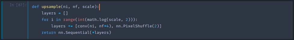
It's one line of code. Here is a conv with number of in to number of filters out times four because we are doing a scale two upsample (2²=4). That's our convolution and then here is our pixel shuffle, it's built into PyTorch. Pixel shuffle is the thing that moves each thing into its right spot. So that will upsample by a scale factor of 2. So we need to do that log base 2 scale times. If scale is four, then we'll do two times to go two times two. So that's what this upsample here does.

Checkerboard pattern [00:44:19]

Great. Guess what. That does not get rid of the checkerboard patterns. We still have checkerboard patterns. So I'm sure in great fury and frustration, the same team from Twitter I think this is back when they used to be a startup called Magic Pony that Twitter bought came back again with another paper saying okay, this time we've got rid of the checkerboard.

Why do we still have a checkerboard? The reason we still have a checkerboard even after doing this is that when we randomly initialize this convolutional kernel at the start, it means that each of these 9 pixels in this little 3x3 grid over here are going to be totally randomly different. But then the next set of 3 pixels will be randomly different to each other but will be very similar to their corresponding pixel in the previous 3x3 section. So we are going to have repeating 3x3 things all the way across. Then as we try to learn something better, it's starting from this repeating 3x3 starting point which is not what we want. What we actually would want is for these 3x3 pixels to be the same to start with. To make these 3x3 pixels the same, we would need to make these 9 channels the same here for each filter. So the solution in this paper is very simple. It's that when we initialize this convolution at start when we randomly initialize it, we don't totally randomly initialize it. We randomly initialize one of the r² sets of channels then we copy that to the other r² so they are all the same. That way, initially, each of these 3x3 will be the same. So that is called ICNR (Initialized to Convolution NN Resize) and that's what we are going to use in a moment.

Pixel loss [00:46:41]

Before we do, let's take a quick look. So we've got this super resolution ResNet which just does lots of computation with lots of ResNet blocks and then it does some upsampling and gets our final three channels out.

Parallelize

Then to make life faster, we are going to run things in parallel. One reason we want to run it in parallel is because Gerardo told us that he has 6 GPUs and this is what his computer looks like right now. 😆

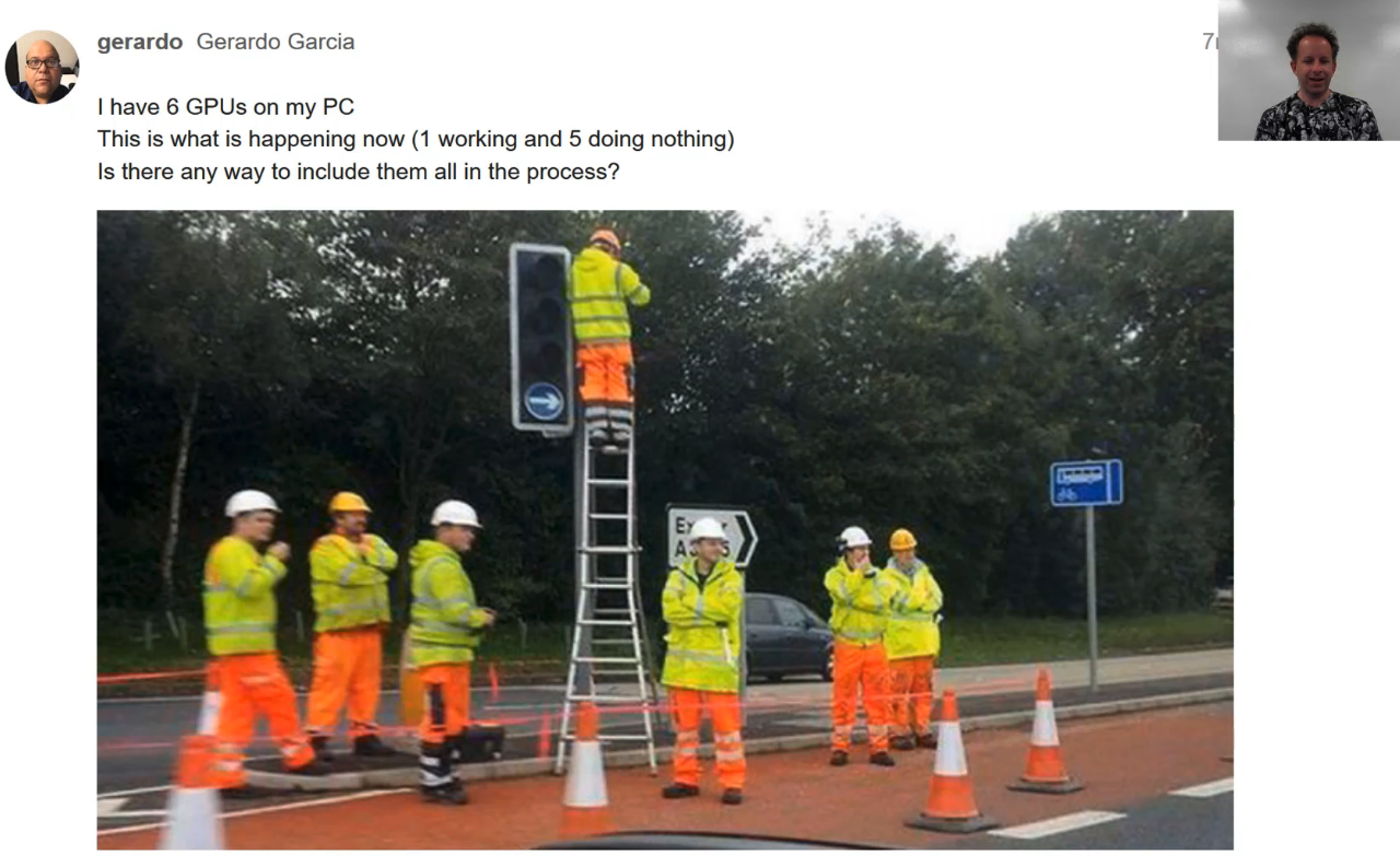
So I'm sure anybody who has more than one GPU has had this experience before. So how do we get these men working together? All you need to do is to take your PyTorch module and wrap it with nn.DataParallel. Once you've done that, it copies it to each of your GPUs and will automatically run it in parallel. It scales pretty well to two GPUs, okay to three GPUs, better than nothing to four GPUs and beyond that, performance does go backwards. By default, it will copy it to all of your GPUs — you can add an array of GPUs otherwise if you want to avoid getting in trouble, for example, I have to share our box with Yannet and if I didn't put this here, then she would be yelling at me right now or boycotting my class. So this is how you avoid getting into trouble with Yannet.

m = to_gpu(SrResnet(64, scale))

# Uncomment this line if you have more than 1 GPU.
m = nn.DataParallel(m, [0, 2])

learn = Learner(md, SingleModel(m), opt_fn=optim.Adam)
learn.crit = F.mse_loss

One thing to be aware of here is that once you do this, it actually modifies your module [00:48:21]. So if you now print out your module, let's say previously it was just an endless sequential, now you'll find it's an nn.Sequential embedded inside a module called Module. In other words, if you save something which you had nn.DataParallel and then tried and load it back into something you haven't nn.DataParallel, it'll say it doesn't match up because one of them is embedded inside this Module attribute and the other one isn't. It may also depend even on which GPU IDs you have had it copy to. Two possible solutions:

1. Don't save the module m but instead save the module attribute m.module because that's actually the non data parallel bit.
2. Always put it on the same GPU IDs and then use data parallel and load and save that every time. That's what I was using.

This is an easy thing for me to fix automatically in fast.ai and I'll do it pretty soon so it will look for that module attribute and deal with it automatically. But for now, we have to do it manually. It's probably useful to know what's going on behind the scenes anyway.

So we've got our module [00:49:46]. I find it'll run 50 or 60% faster on a 1080 Ti, if you are running on Volta, it actually parallelize a bit better. There are much faster ways to parallelize but this is a super easy way.

Loss function and training

We create our learner in the usual way. We can use MSE loss here so that's just going to compare the pixels of the output to the pixels that we expected. We can run our learning rate finder and we can train it for a while.

learn.lr_find(start_lr=1e-5, end_lr=10000)
learn.sched.plot(10, 0)

# -----------------------------------------------------------------------------
# Output
# -----------------------------------------------------------------------------
30%|███       | 183/602 [03:10<07:17,  1.04s/it, loss=9.88]

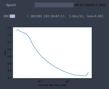
lr = 2e-3
learn.fit(lr, 1, cycle_len=1, use_clr_beta=(40, 10))

# -----------------------------------------------------------------------------
# Output
# -----------------------------------------------------------------------------
Epoch 100% 1/1 [09:48<00:00, 588.53s/it]

epoch      trn_loss   val_loss
    0      0.103036   0.09909
[array([0.09909])]

x,y = next(iter(md.val_dl))
preds = learn.model(VV(x))

Here is our input:

idx = 1
show_img(y, idx, normed=True)

And here is our output.

show_img(preds, idx, normed=True)

And you can see that what we've managed to do is to train a very advanced residual convolutional network that's learnt to blur things. Why is that? Well, because it's what we asked for. We said to minimize MSE loss. MSE loss between pixels really the best way to do that is just average the pixel i.e. to blur it. So that's why pixel loss is no good. So we want to use our perceptual loss.

show_img(x, idx, normed=True)

idx = 2

# Ground truth image (high-res)
show_img(y, idx, normed=True)

# # Upsampled image (output)
show_img(preds, idx, normed=True)

# Input image (low-res)
show_img(x, idx, normed=True)

Perceptual loss [00:50:57]

With perceptual loss, we are basically going to take our VGG network and just like we did last week, we are going to find the block index just before we get a maxpool.

def icnr(x, scale=2, init=nn.init.kaiming_normal):
    new_shape = [int(x.shape[0] / (scale ** 2))] + list(x.shape[1:])
    subkernel = torch.zeros(new_shape)
    subkernel = init(subkernel)
    subkernel = subkernel.transpose(0, 1)
    subkernel = subkernel.contiguous().view(subkernel.shape[0],
                                            subkernel.shape[1], -1)
    kernel = subkernel.repeat(1, 1, scale ** 2)
    transposed_shape = [x.shape[1]] + [x.shape[0]] + list(x.shape[2:])
    kernel = kernel.contiguous().view(transposed_shape)
    kernel = kernel.transpose(0, 1)
    return kernel

m_vgg = vgg16(True)

blocks = [i - 1 for i, o in enumerate(children(m_vgg))
                    if isinstance(o, nn.MaxPool2d)]
blocks, [m_vgg[i] for i in blocks]

# -----------------------------------------------------------------------------
# Output
# -----------------------------------------------------------------------------
([5, 12, 22, 32, 42],
 [ReLU(inplace), ReLU(inplace), ReLU(inplace), ReLU(inplace), ReLU(inplace)])

So here are the ends of each block of the same grid size. If we just print them out, as we'd expect, every one of those is a ReLU module and so in this case these last two blocks are less interesting to us. The grid size there is small enough, and course enough that it's not as useful for super resolution. So we are just going to use the first three. Just to save unnecessary computation, we are just going to use those first 23 layers of VGG and we'll throw away the rest. We'll stick it on the GPU. We are not going to be training this VGG model at all — we are just using it to compare activations. So we'll stick it in eval mode and we will set it to not trainable.

vgg_layers = children(m_vgg)[:23]
m_vgg = nn.Sequential(*vgg_layers).cuda().eval()
set_trainable(m_vgg, False)

def flatten(x): return x.view(x.size(0), -1)

Just like last week, we will use SaveFeatures class to do a forward hook which saves the output activations at each of those layers [00:52:07].

class SaveFeatures():
    features=None
    def __init__(self, m): self.hook = m.register_forward_hook(self.hook_fn)
    def hook_fn(self, module, input, output): self.features = output
    def remove(self): self.hook.remove()

So now we have everything we need to create our perceptual loss or as I call it here FeatureLoss class. We are going to pass in a list of layer IDs, the layers where we want the content loss to be calculated, and a list of weights for each of those layers. We can go through each of those layer IDs and create an object which has the forward hook function to store the activations. So in our forward, then we can just go ahead and call the forward pass of our model with the target (high res image we are trying to create). The reason we do that is because that is going to then call that hook function and store in self.sfs (self dot save features) the activations we want. Now we are going to need to do that for our conv net output as well. So we need to clone these because otherwise the conv net output is going to go ahead and just clobber what I already had. So now we can do the same thing for the conv net output which is the input to the loss function. And so now we've got those two things we can zip them all together along with the weights so we've got inputs, targets, and weights. Then we can do the L1 loss between the inputs and the targets and multiply by the layer weights. The only other thing I do is I also grab the pixel loss, but I weight it down quite a bit. Most people don't do this. I haven't seen papers that do this, but in my opinion, it's maybe a little bit better because you've got the perceptual content loss activation stuff but the really finest level it also cares about the individual pixels. So that's our loss function.

class FeatureLoss(nn.Module):
    def __init__(self, m, layer_ids, layer_wgts):
        super().__init__()
        self.m, self.wgts = m, layer_wgts
        self.sfs = [SaveFeatures(m[i]) for i in layer_ids]

    def forward(self, input, target, sum_layers=True):
        self.m(VV(target.data))
        res = [F.l1_loss(input, target) / 100]
        targ_feat = [V(o.features.data.clone()) for o in self.sfs]
        self.m(input)
        res += [F.l1_loss(flatten(inp.features), flatten(targ)) * wgt
               for inp, targ, wgt in zip(self.sfs, targ_feat, self.wgts)]
        if sum_layers: res = sum(res)
        return res

    def close(self):
        for o in self.sfs: o.remove()

We create our super resolution ResNet telling it how much to scale up by.

m = SrResnet(64, scale)

And then we are going to do our icnr initialization of that pixel shuffle convolution [00:54:27]. This is very boring code, I actually stole it from somebody else. Literally all it does is just say okay, you've got some weight tensor x that you want to initialize so we are going to treat it as if it has shape (i.e. number of features) divided by scale squared features in practice. So this might be 2² = 4 because we actually want to just keep one set of then and then copy them four times, so we divide it by four and we create something of that size and we initialize that with, by default, kaiming_normal initialization. Then we just make scale² copies of it. And the rest of it is just kind of moving axes around a little bit. So that's going to return a new weight matrix where each initialized sub kernel is repeated r² or scale² times. So that details don't matter very much. All that matters here is that I just looked through to find what was the actual conv layer just before the pixel shuffle and store it away and then I called icnr on its weight matrix to get my new weight matrix. And then I copied that new weight matrix back into that layer.

conv_shuffle = m.features[10][0][0]
kernel = icnr(conv_shuffle.weight, scale=scale)
conv_shuffle.weight.data.copy_(kernel)

As you can see, I went to quite a lot of trouble in this exercise to really try to implement all the best practices [00:56:13]. I tend to do things a bit one extreme or the other. I show you a really hacky version that only slightly works or I go to the nth degree to make it work really well. So this is a version where I'm claiming that this is pretty much a state of the art implementation. It's a competition winning or at least my re-implementation of a competition winning approach. The reason I'm doing that is because I think this is one of those rare papers where they actually get a lot of the details right and I want you to get a feel of what it feels like to get all the details right. Remember, getting the details right is the difference between the hideous blurry mess and the pretty exquisite result.

m = to_gpu(m)

learn = Learner(md, SingleModel(m), opt_fn=optim.Adam)

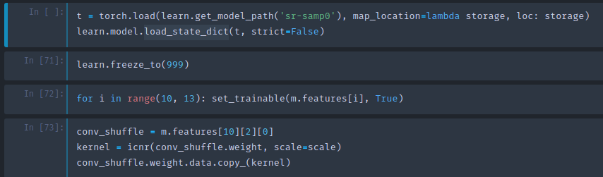
t = torch.load(learn.get_model_path('sr-samp0'),
         map_location=lambda storage, loc: storage)
learn.model.load_state_dict(t, strict=False)

learn.freeze_to(999)

for i in range(10, 13): set_trainable(m.features[i], True)

conv_shuffle = m.features[10][2][0]
kernel = icnr(conv_shuffle.weight, scale=scale)
conv_shuffle.weight.data.copy_(kernel)

So we are going do DataParallel on that again [00:57:14].

# m = nn.DataParallel(m, [0, 2])

learn = Learner(md, SingleModel(m), opt_fn=optim.Adam)

learn.set_data(md)

We are going to set our criterion to be FeatureLoss using our VGG model, grab the first few blocks and these are sets of layer weights that I found worked pretty well.

learn.crit = FeatureLoss(m_vgg, blocks[:3], [0.2, 0.7, 0.1])

lr = 6e-3
wd = 1e-7

Do a learning rate finder.

%time learn.lr_find(1e-4, 0.1, wds=wd, linear=True)

# -----------------------------------------------------------------------------
# Output
# -----------------------------------------------------------------------------
12%|█▏        | 71/602 [03:10<23:44,  2.68s/it, loss=0.807]
CPU times: user 4min 32s, sys: 17.9 s, total: 4min 50s
Wall time: 3min 10s

learn.sched.plot(n_skip_end=1)

Fit it for a while.

learn.fit(lr, 1, cycle_len=2, wds=wd, use_clr=(20, 10))

# -----------------------------------------------------------------------------
# Output
# -----------------------------------------------------------------------------
Epoch 100% 2/2 [52:34<00:00, 1577.27s/it]

epoch      trn_loss   val_loss
    0      0.06387    0.062875
    1      0.062231   0.060575
[array([0.06057])]

learn.save('sr-samp0')

And I fiddled around for a while trying to get some of these details right. But here is my favorite part of the paper is what happens next. Now that we've done it for scale equals 2 — progressive resizing. So progressive resizing is the trick that let us get the best best single computer result for ImageNet training on DAWNBench. It's this idea of starting small gradually making bigger. I only know of two papers that have used this idea. One is the progressive resizing of GANs paper which allows training a very high resolution GANs and the other one is the EDSR paper. And the cool thing about progressive resizing is not only are your earlier epochs, assuming you've got 2x2 smaller, four times faster. You can also make the batch size maybe 3 or 4 times bigger. But more importantly, they are going to generalize better because you are feeding in your model different sized images during training. So we were able to train half as many epochs for ImageNet as most people. Our epochs were faster and there were fewer of them. So progressive resizing is something that, particularly if you are training from scratch (I'm not so sure if it's useful for fine-tuning transfer learning, but if you are training from scratch), you probably want to do nearly all the time.

Progressive resizing [00:59:07]

So the next step is to go all the way back to the top and change to 4 scale, 32 batch size, restart. I saved the model before I do that.

Go back and that's why there's a little bit of fussing around in here with reloading because what I needed to do now is I needed to load my saved model back in.

But there's a slight issue which is I now have one more upsampling layer than I used to have to go from 2x2 to 4x4. My loop here is now looping through twice, not once. Therefore, it's added an extra conv net and an extra pixel shuffle. So how am I going to load in weights for a different network?

The answer is that I use a very handy thing in PyTorch load_state_dict. This is what learner.load calls behind the scenes. If I pass this parameter strict=False then it says "okay, if you can't fill in all of the layers, just fill in the layers you can." So after loading the model back in this way, we are going to end up with something where it's loaded in all the layers that it can and that one conv layer that's new is going to be randomly initialized.

Then I freeze all my layers and then unfreeze that upsampling part [1:00:45] Then use icnr on my newly added extra layer. Then I can go ahead and learn again. So then the rest is the same.

If you are trying to replicate this, don't just run this top to bottom. Realize it involves a bit of jumping around.

learn.load('sr-samp1')

lr = 3e-3

learn.fit(lr, 1, cycle_len=1, wds=wd, use_clr=(20, 10))

# -----------------------------------------------------------------------------
# Output
# -----------------------------------------------------------------------------
epoch      trn_loss   val_loss
    0      0.069054   0.06638
[array([0.06638])]

learn.save('sr-samp2')

learn.unfreeze()

learn.load('sr-samp2')

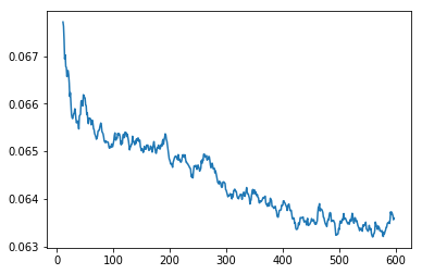
learn.fit(lr / 3, 1, cycle_len=1, wds=wd, use_clr=(20, 10))

# -----------------------------------------------------------------------------
# Output
# -----------------------------------------------------------------------------
Epoch 100% 1/1 [26:22<00:00, 1582.05s/it]

epoch      trn_loss   val_loss
    0      0.063521   0.060426
[array([0.06043])]

learn.save('sr1')

learn.sched.plot_loss()

def plot_ds_img(idx, ax=None, figsize=(7, 7), normed=True):
    if ax is None: fig, ax = plt.subplots(figsize=figsize)
    im = md.val_ds[idx][0]
    if normed: im = denorm(im)[0]
    else:      im = np.rollaxis(to_np(im), 0, 3)
    ax.imshow(im)
    ax.axis('off')

fig, axes = plt.subplots(6, 6, figsize=(20, 20))
for i, ax in enumerate(axes.flat):
    plot_ds_img(i + 35, ax=ax, normed=True)

x, y = md.val_ds[215]

y = y[None]

learn.model.eval()
preds = learn.model(VV(x[None]))
x.shape, y.shape, preds.shape

# -----------------------------------------------------------------------------
# Output
# -----------------------------------------------------------------------------
((3, 72, 72), (1, 3, 288, 288), torch.Size([1, 3, 288, 288]))

learn.crit(preds, V(y), sum_layers=False)

# -----------------------------------------------------------------------------
# Output
# -----------------------------------------------------------------------------
[Variable containing:
 1.00000e-03 *
   1.3694
 [torch.cuda.FloatTensor of size 1 (GPU 0)], Variable containing:
 1.00000e-02 *
   1.0221
 [torch.cuda.FloatTensor of size 1 (GPU 0)], Variable containing:
 1.00000e-02 *
   3.9270
 [torch.cuda.FloatTensor of size 1 (GPU 0)], Variable containing:
 1.00000e-03 *
   3.9834
 [torch.cuda.FloatTensor of size 1 (GPU 0)]]

learn.crit.close()

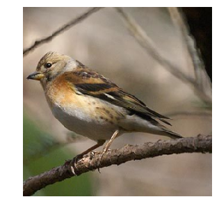
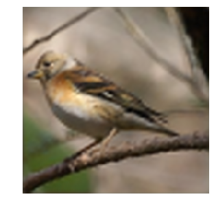
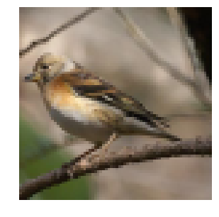
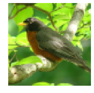
The longer you train, the better it gets [1:01:18]. I ended up training it for about 10 hours, but you'll still get very good results much more quickly if you're less patient. So we can try it out and and here is the result. On the left is my pixelated bird and on the right is the upsampled version. It literally invented coloration. But it figured out what kind of bird it is, and it knows what these feathers are meant to look like. So it has imagined a set of feathers which are compatible with these exact pixels which is genius. Same for the back of its head. There is no way you can tell what these blue dots are meant to represent. But if you know that this kind of bird has an array of feathers here, you know that's what they must be. Then you can figure out whether the feathers would have to be such that when they were pixelated they would end up in these spots. So it literally reverse engineered given its knowledge of this exact species of bird, how it would have to have looked to create this output. This is so amazing. It also knows from all the signs around it that this area here (background) was almost certainly blurred out. So it actually reconstructed blurred vegetation. If it hadn't have done all of those things, it wouldn't have gotten such a good loss function. Because in the end, it had to match the activations saying "oh, there's a feather over here and it's kind of fluffy looking and it's in this direction" and all that.

_, axes = plt.subplots(1, 2, figsize=(14, 7))
show_img(x[None], 0, ax=axes[0])
show_img(preds, 0, normed=True, ax=axes[1])

Well, that brings us to the end of super resolution [1:03:18]. Don't forget to check out the ask Jeremy anything thread.

Ask Jeremy Anything

❓ What are the future plans for fast.ai and this course? Will there be a part 3? If there is a part 3, I would really love to take it [1:04:11].

Jeremy: I'm not quite sure. It's always hard to guess. I hope there will be some kind of follow-up. Last year, after part 2, one of the students started up a weekly book club going through the Ian Goodfellow Deep Learning book, and Ian actually came in and presented quite a few of the chapters and there was somebody, an expert, who presented every chapter. That was a really cool part 3. To a large extent, it will depend on you, the community, to come up with ideas and help make them happen, and I'm definitely keen to help. I've got a bunch of ideas but I'm nervous about saying them because I'm not sure which ones will happen and which ones won't. But the more support I have in making things happen that you want to happen from you, the more likely they are to happen.

❓ What was your experience like starting down the path of entrepreneurship? Have you always been an entrepreneur or did you start at a big company and transition to a startup? Did you go from academia to startups or startups to academia? [1:05:13]

Jeremy: No, I was definitely not an academia. I am totally a fake academic. I started at McKinsey and company which is a strategy firm when I was 18 which meant I couldn't really go to university so it didn't really turn up. Then spent 8 years in business helping really big companies on strategic questions. I always wanted to be an entrepreneur, planned to only spend two years in McKinsey, only thing I really regret in my life was not sticking to that plan and wasting eight years instead. So two years would have been perfect. But then I went into entrepreneurship, started two companies in Australia. The best part about that was that I didn't get any funding so all the money that I made was mine or the decisions were mine and my partner's. I focused entirely on profit and product and customer and service. Whereas I find in San Francisco, I'm glad I came here and so the two of us came here for Kaggle, Anthony and I, and raised ridiculous amount of money 11 million dollar for this really new company. That was really interesting but it's also really distracting trying to worry about scaling and VC's wanting to see what your business development plans are and also just not having any real need to actually make a profit. So I had a bit of the same problem at Enlitic where I again raised a lot of money 15 million dollars pretty quickly and a lot of distractions. I think trying to bootstrap your own company and focus on making money by selling something at a profit and then plowing that back into the company, it worked really well. Because within five years, we were making a profit from 3 months in and within 5 years, we were making enough for profit not just to pay all of us and our own wages but also to see my bank account growing and after 10 years sold it for a big chunk of money, not enough that a VC would be excited but enough that I didn't have to worry about money again. So I think bootstrapping a company is something which people in the Bay Area at least don't seem to appreciate how good of an idea that is.

❓ If you were 25 years old today and still know what you know where would you be looking to use AI? What are you working on right now or looking to work on in the next 2 years [1:08:10]?

Jeremy: You should ignore the last part of that. I won't even answer it. Doesn't matter where I'm looking. What you should do is leverage your knowledge about your domain. So one of the main reasons we do this is to get people who have backgrounds in recruiting, oil field surveys, journalism, activism, whatever and solve your problems. It'll be really obvious to you what real problems are and it will be really obvious to you what data you have and where to find it. Those are all the bits that for everybody else that's really hard. So people who start out with "oh, I know deep learning now I'll go and find something to apply it to" basically never succeed where else people who are like "oh, I've been spending 25 years doing specialized recruiting for legal firms and I know that the key issue is this thing and I know that this piece of data totally solves it and so I'm just going to do that now and I already know who to call or actually start selling it to". They are the ones who tend to win. If you've done nothing but academic stuff, then it's more maybe about your hobbies and interests. So everybody has hobbies. The main thing I would say is please don't focus on building tools for data scientists to use or for software engineers to use because every data scientist knows about the market of data scientists whereas only you know about the market for analyzing oil survey world or understanding audiology studies or whatever it is that you do.

❓ Given what you've shown us about applying transfer learning from image recognition to NLP, there looks to be a lot of value in paying attention to all of the developments that happen across the whole ML field and that if you were to focus in one area you might miss out on some great advances in other concentrations. How do you stay aware of all of the advancements across the field while still having time to dig in deep to your specific domains [1:10:19]?

Jeremy: Yeah, that's awesome. I mean that's one of the key messages of this course. Lots of good work's being done in different places and people are so specialized and most people don't know about it. If I can get state of the art results in NLP within six months of starting to look at NLP and I think that says more about NLP than it does about me, frankly. It's kind of like the entrepreneurship thing. You pick the areas you see that you know about and kind of transfer stuff like "oh, we could use deep learning to solve this problem" or in this case, we could use this idea of computer vision to solve that problem. So things like transfer learning, I'm sure there's like a thousand opportunities for you to do in other field to do what Sebastian and I did in NLP with NLP classification. So the short answer to your question is the way to stay ahead of what's going on would be to follow my feed of Twitter favorites and my approach is to then follow lots and lots of people on Twitter and put them into the Twitter favorites for you. Literally, every time I come across something interesting, I click favorite. There are two reasons I do it. The first is that when the next course comes along, I go through my favorites to find which things I want to study. The second is so that you can do the same thing. And then which you go deep into, it almost doesn't matter. I find every time I look at something it turns out to be super interesting and important. So pick something which you feel like solving that problem would be actually useful for some reason and it doesn't seem to be very popular which is kind of the opposite of what everybody else does. Everybody else works on the problems which everybody else is already working on because they are the ones that seem popular. I can't quite understand this train of thinking but it seems to be very common.

❓ Is Deep Learning an overkill to use on Tabular data? When is it better to use DL instead of ML on tabular data [1:12:46]?

Jeremy: Is that a real question or did you just put that there so that I would point out that Rachel Thomas just wrote an article? http://www.fast.ai/2018/04/29/categorical-embeddings/

So Rachel has just written about this and Rachel and I spent a long time talking about it and the short answer is we think it's great to use deep learning on tabular data. Actually, of all the rich complex important and interesting things that appear in Rachel's Twitter stream covering everything from the genocide of Rohingya through to latest ethics violations in AI companies, the one by far that got the most attention and engagement from the community was the question about is it called tabular data or structured data. So yeah, ask computer people how to name things and you'll get plenty of interest. There are some really good links here to stuff from Instacart and Pinterest and other folks who have done some good work in this area. Any of you that went to the Data Institute conference would have seen Jeremy Stanley's presentation about the really cool work they did at Instacart.

Rachel: I relied heavily on lessons 3 and 4 from part 1 in writing this post so much of that may be familiar to you.

Jeremy: Rachel asked me during the post like how to tell whether you should use the decision tree ensemble like GBM or random forest or neural net and my answer is I still don't know. Nobody I'm aware of has done that research in any particularly meaningful way. So there's a question to be answered there, I guess. My approach has been to try to make both of those things as accessible as possible through fast.ai library so you can try them both and see what works. That's what I do.

❓ Reinforcement Learning popularity has been on a gradual rise in the recent past. What's your take on Reinforcement Learning? Would fast.ai consider covering some ground in popular RL techniques in the future [1:15:21]?

Jeremy: I'm still not a believer in reinforcement learning. I think it's an interesting problem to solve but it's not at all clear that we have a good way of solving this problem. So the problem, it really is the delayed credit problem. So I want to learn to play pong, I've moved up or down and three minutes later I find out whether I won the game of pong — which actions I took were actually useful? So to me, the idea of calculating the gradients of the output with respect to those inputs, the credit is so delayed that those derivatives don't seem very interesting. I get this question quite regularly in every one of these four courses so far. I've always said the same thing. I'm rather pleased that finally recently there's been some results showing that actually basically random search often does better than reinforcement learning so basically what's happened is very well-funded companies with vast amounts of computational power throw all of it at reinforcement learning problems and get good results and people then say "oh it's because of the reinforcement learning" rather than the vast amounts of compute power. Or they use extremely thoughtful and clever algorithms like a combination of convolutional neural nets and Monte Carlo tree search like they did with the Alpha Go stuff to get great results and people incorrectly say "oh that's because of reinforcement learning" when it wasn't really reinforcement learning at all. So I'm very interested in solving these kind of more generic optimization type problems rather than just prediction problems and that's what these delayed credit problems tend to look like. But I don't think we've yet got good enough best practices that I have anything on, ready to teach and say I've got to teach you this thing because I think it's still going to be useful next year. So we'll keep watching and see what happens.

Super resolution network to a style transfer network [01:17:57]

We are going to now turn the super resolution network into a style transfer network. And we'll do this pretty quickly. We basically already have something. x is my input image and I'm going to have some loss function and I've got some neural net again. Instead of a neural net that does a whole a lot of compute and then does upsampling at the end, our input this time is just as big as our output. So we are going to do some downsampling first. Then our computer, and then our upsampling. So that's the first change we are going to make — we are going to add some downsampling so some stride 2 convolution layers to the front of our network. The second is rather than just comparing yc and x are the same thing here. So we are going to basically say our input image should look like itself by the end. Specifically we are going to compare it by chucking it through VGG and comparing it at one of the activation layers. And then its style should look like some painting which we'll do just like we did with the Gatys' approach by looking at the Gram matrix correspondence at a number of layers. So that's basically it. So that ought to be super straight forward. It's really combining two things we've already done.

Style transfer network [01:19:19]

Notebook

So all this code starts identical, except we don't have high res and low res, we just have one size 256.

%matplotlib inline
%reload_ext autoreload
%autoreload 2

from fastai.conv_learner import *
from pathlib import Path
# torch.cuda.set_device(0)

torch.backends.cudnn.benchmark = True

PATH = Path('data/imagenet')
PATH_TRN = PATH / 'train'

fnames_full, label_arr_full, all_labels = folder_source(PATH, 'train')
fnames_full = ['/'.join(Path(fn).parts[-2:]) for fn in fnames_full]
list(zip(fnames_full[:5], label_arr_full[:5]))

# -----------------------------------------------------------------------------
# Output
# -----------------------------------------------------------------------------
[('n01440764/n01440764_12241.JPEG', 0),
 ('n01440764/n01440764_529.JPEG', 0),
 ('n01440764/n01440764_11155.JPEG', 0),
 ('n01440764/n01440764_9649.JPEG', 0),
 ('n01440764/n01440764_8013.JPEG', 0)]

all_labels[:5]

# -----------------------------------------------------------------------------
# Output
# -----------------------------------------------------------------------------
['n01440764', 'n01443537', 'n01491361', 'n01494475', 'n01498041']

np.random.seed(42)
keep_pct = 1.
# keep_pct = 0.1
keeps = np.random.rand(len(fnames_full)) < keep_pct
fnames = np.array(fnames_full, copy=False)[keeps]
label_arr = np.array(label_arr_full, copy=False)[keeps]

arch = vgg16

# sz, bs = 96, 32
sz, bs = 256, 24
# sz, bs = 128, 32

class MatchedFilesDataset(FilesDataset):
    def __init__(self, fnames, y, transform, path):
        self.y = y
        assert(len(fnames) == len(y))
        super().__init__(fnames, transform, path)

    def get_y(self, i): return open_image(os.path.join(self.path, self.y[i]))

    def get_c(self): return 0

val_idxs = get_cv_idxs(len(fnames), val_pct=min(0.01/keep_pct, 0.1))
((val_x, trn_x), (val_y, trn_y)) = split_by_idx(val_idxs, np.array(fnames), np.array(fnames))
len(val_x), len(trn_x)

# -----------------------------------------------------------------------------
# Output
# -----------------------------------------------------------------------------
(194, 19245)

img_fn = PATH / 'train' / 'n01558993' / 'n01558993_9684.JPEG'

tfms = tfms_from_model(arch, sz, tfm_y=TfmType.PIXEL)
datasets = ImageData.get_ds(MatchedFilesDataset, (trn_x, trn_y), (val_x, val_y), tfms, path=PATH_TRN)
md = ImageData(PATH, datasets, bs, num_workers=16, classes=None)

denorm = md.val_ds.denorm

def show_img(ims, idx, figsize=(5, 5), normed=True, ax=None):
    if ax is None: fig, ax = plt.subplots(figsize=figsize)
    if normed: ims = denorm(ims)
    else:      ims = np.rollaxis(to_np(ims), 1, 4)
    ax.imshow(np.clip(ims, 0, 1)[idx])
    ax.axis('off')

Model [01:19:30]

My model is the same. One thing I did here is I did not do any kind of fancy best practices for this one at all. Partly because there doesn't seem to be any. There's been very little follow up in this approach compared to the super resolution stuff. We'll talk about why in a moment. So you'll see, this is much more normal looking.

def conv(ni, nf, kernel_size=3, stride=1, actn=True, pad=None, bn=True):
    if pad is None: pad = kernel_size//2
    layers = [nn.Conv2d(ni, nf, kernel_size, stride=stride, padding=pad, bias=not bn)]
    if actn: layers.append(nn.ReLU(inplace=True))
    if bn: layers.append(nn.BatchNorm2d(nf))
    return nn.Sequential(*layers)

I've got batch norm layers. I don't have scaling factor here.

class ResSequentialCenter(nn.Module):
    def __init__(self, layers):
        super().__init__()
        self.m = nn.Sequential(*layers)

    def forward(self, x): return x[:, :, 2:-2, 2:-2] + self.m(x)

def res_block(nf):
    return ResSequentialCenter([conv(nf, nf, actn=True, pad=0), conv(nf, nf, pad=0)])

I don't have a pixel shuffle — it's just using a normal upsampling followed by 1x1 conf. So it's just more normal.

def upsample(ni, nf):
    return nn.Sequential(nn.Upsample(scale_factor=2), conv(ni, nf))

One thing they mentioned in the paper is they had a lot of problems with zero padding creating artifacts and the way they solved that was by adding 40 pixel of reflection padding at the start. So I did the same thing and then they used zero padding in their convolutions in their Res blocks. Now if you've got zero padding in your convolutions in your Res blocks, then that means that the two parts of your ResNet won't add up anymore because you've lost a pixel from each side on each of your two convolutions. So my ResSequential has become ResSequentialCenter and I've removed the last 2 pixels on each side of those good cells. Other than that, this is basically the same as what we had before.

class StyleResnet(nn.Module):
    def __init__(self):
        super().__init__()
        features = [
            nn.ReflectionPad2d(40),
            conv(3, 32, 9),
            conv(32, 64, stride=2),
            conv(64, 128, stride=2)
        ]
        for i in range(5):
            features.append(res_block(128))
        features += [
            upsample(128, 64),
            upsample(64, 32),
            conv(32, 3, 9, actn=False)
        ]
        self.features = nn.Sequential(*features)

    def forward(self, x):
        return self.features(x)

Style Image [01:21:02]

So then we can bring in our starry night picture.

style_fn = PATH / 'style' / 'starry_night.jpg'
style_img = open_image(style_fn)
style_img.shape

# -----------------------------------------------------------------------------
# Output
# -----------------------------------------------------------------------------
(900, 1136, 3)

plt.imshow(style_img)

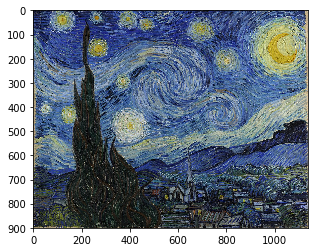
h, w, _ = style_img.shape
rat = max(sz / h, sz / h)
res = cv2.resize(style_img, (int(w * rat), int(h * rat)), interpolation=cv2.INTER_AREA)
resz_style = res[:sz, -sz:]

We can resize it.

plt.imshow(resz_style)

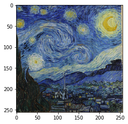
We can throw it through our transformations.

style_tfm, _ = tfms[1](resz_style, resz_style)

style_tfm = np.broadcast_to(style_tfm[None], (bs,) + style_tfm.shape)

Just to make the method a little bit easier for my brain to handle, I took our transform style image which after transformations of 3 x 256 x 256, and I made a mini batch. My batch size is 24 — 24 copies of it. It just makes it a little bit easier to do the kind of batch arithmetic without worrying about some of the broadcasting. They are not really 24 copies. I used np.broadcast to basically fake 24 pieces.

style_tfm.shape

# -----------------------------------------------------------------------------
# Output
# -----------------------------------------------------------------------------
(24, 3, 256, 256)

Perceptual loss [01:21:51]

So just like before, we create a VGG, grab the last block. This time we are going to use all of these layers so we keep everything up to the 43rd layer.

m_vgg = vgg16(True)

blocks = [i - 1 for i, o in enumerate(children(m_vgg))
                    if isinstance(o, nn.MaxPool2d)]
blocks, [m_vgg[i] for i in blocks[1:]]

# -----------------------------------------------------------------------------
# Output
# -----------------------------------------------------------------------------
([5, 12, 22, 32, 42],
 [ReLU(inplace), ReLU(inplace), ReLU(inplace), ReLU(inplace)])

vgg_layers = children(m_vgg)[:43]
m_vgg = nn.Sequential(*vgg_layers).cuda().eval()
set_trainable(m_vgg, False)

def flatten(x): return x.view(x.size(0), -1)

class SaveFeatures():
    features = None
    def __init__(self, m): self.hook = m.register_forward_hook(self.hook_fn)
    def hook_fn(self, module, input, output): self.features = output
    def remove(self): self.hook.remove()

def ct_loss(input, target): return F.mse_loss(input, target)

def gram(input):
    b, c, h, w = input.size()
    x = input.view(b, c, -1)
    return torch.bmm(x, x.transpose(1, 2)) / (c * h * w) *1e6

def gram_loss(input, target):
    return F.mse_loss(gram(input), gram(target[:input.size(0)]))

So now our combined loss is going to add together a content loss for the third block plus the Gram loss for all of our blocks with different weights. Again, going back to everything being as normal as possible, I've gone back to using MSE above. Basically what happened was I had a lot of trouble getting this to train properly. So I gradually removed trick after trick and eventually just went "ok, I'm just gonna make it as bland as possible".

📝 Last week's Gram matrix was wrong, by the way [1:22:37]. It only worked for a batch size of one and we only had a batch size of one so that was fine. I was using matrix multiply which meant that every batch was being compared to every other batch. You actually need to use batch matrix multiple (torch.bmm) which does a matrix multiply per batch. So that's something to be aware of there.

class CombinedLoss(nn.Module):
    def __init__(self, m, layer_ids, style_im, ct_wgt, style_wgts):
        super().__init__()
        self.m, self.ct_wgt, self.style_wgts = m, ct_wgt, style_wgts
        self.sfs = [SaveFeatures(m[i]) for i in layer_ids]
        m(VV(style_im))
        self.style_feat = [V(o.features.data.clone()) for o in self.sfs]

    def forward(self, input, target, sum_layers=True):
        self.m(VV(target.data))
        targ_feat = self.sfs[2].features.data.clone()
        self.m(input)
        inp_feat = [o.features for o in self.sfs]

        res = [ct_loss(inp_feat[2], V(targ_feat)) * self.ct_wgt]
        res += [gram_loss(inp, targ) * wgt for inp, targ, wgt
                in zip(inp_feat, self.style_feat, self.style_wgts)]

        if sum_layers: res = sum(res)
        return res

    def close(self):
        for o in self.sfs: o.remove()

So I've got Gram matrices, I do my MSE loss between the Gram matrices, I weight them by style weights, so I create that ResNet.

m = StyleResnet()
m = to_gpu(m)

learn = Learner(md, SingleModel(m), opt_fn=optim.Adam)

I create my combined loss passing in the VGG network, passing in the block IDs, passing in the transformed starry night image, and you'll see the the very start here, I do a forward pass through my VGG model with that starry night image in order that I can save the features for it. Notice, it's really important now that I don't do any data augmentation because I've saved the style features for a particular non-augmented version. So if I augmented it, it might make some minor problems. But that's fine because I've got all of ImageNet to deal with. I don't really need to do data augmentation anyway.

learn.crit = CombinedLoss(m_vgg, blocks[1:], style_tfm, 1e4, [0.025, 0.275, 5., 0.2])

wd = 1e-7

learn.lr_find(wds=wd)
learn.sched.plot(n_skip_end=1)

# -----------------------------------------------------------------------------
# Output
# -----------------------------------------------------------------------------
49%|████▊     | 390/802 [16:33<17:29,  2.55s/it, loss=1.86e+06]

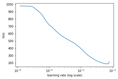
lr = 5e-3

So I've got my loss function and I can go ahead and fit [1:24:06]. And there is nothing clever here at all.

%time learn.fit(lr, 1, cycle_len=1, wds=wd, use_clr=(20, 10))

# -----------------------------------------------------------------------------
# Output
# -----------------------------------------------------------------------------
Epoch 100% 1/1 [33:40<00:00, 2020.41s/it]

epoch      trn_loss   val_loss
    0      116.030613 115.316882
CPU times: user 37min 11s, sys: 2min 50s, total: 40min 2s
Wall time: 33min 40s
[array([115.31688])]

learn.save('style-transfer-net-1')

x, y = md.val_ds[1]

learn.model.eval()
preds = learn.model(VV(x[None]))
x.shape, y.shape, preds.shape

# -----------------------------------------------------------------------------
# Output
# -----------------------------------------------------------------------------
((3, 256, 256), (3, 256, 256), torch.Size([1, 3, 256, 256]))

At the end, I have my sum_layers=False so I can see what each part looks like and see they are balanced. And I can finally pop it out.

learn.crit(preds, VV(y[None]), sum_layers=False)

# -----------------------------------------------------------------------------
# Output
# -----------------------------------------------------------------------------
[Variable containing:
  61.2578
 [torch.cuda.FloatTensor of size 1 (GPU 0)], Variable containing:
  3.3731
 [torch.cuda.FloatTensor of size 1 (GPU 0)], Variable containing:
  4.3279
 [torch.cuda.FloatTensor of size 1 (GPU 0)], Variable containing:
  4.6045
 [torch.cuda.FloatTensor of size 1 (GPU 0)], Variable containing:
  41.2980
 [torch.cuda.FloatTensor of size 1 (GPU 0)]]

learn.crit.close()

_, axes = plt.subplots(1, 2, figsize=(14, 7))
show_img(x[None], 0, ax=axes[0])
show_img(preds, 0, normed=True, ax=axes[1])

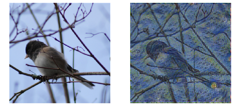
So I mentioned that should be pretty easy and yet it took me about 4 days because I just found this incredibly fiddly to actually get it to work [1:24:26]. So when I finally got up in the morning I said to Rachel "guess what, it trained correctly." Rachel said "I never thought that was going to happen." It just looked awful all the time and it's really about getting the exact right mix of content loss and a style loss and the mix of the layers of the style loss. The worst part was it takes a really long time to train the darn CNN and I didn't really know how long to train it before I decided it wasn't doing well. Should I just train it for longer? And I don't know all the little details didn't seem to slightly change it but just it would totally fall apart all the time. So I kind of mentioned this partly to say just remember the final answer you see here is after me driving myself crazy all week of nearly always not working until finally the last minute it finally does. Even for things which just seemed like they couldn't possibly be difficult because that is combining two things we already have working. The other is to be careful about how we interpret what authors claim.

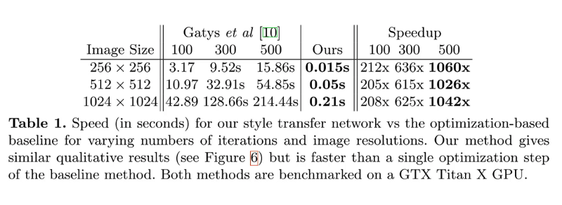
It was so fiddly getting this style transfer to work [1:26:10]. After doing it, it left me thinking why did I bother because now I've got something that takes hours to create a network that can turn any kind of photo into one specific style. It just seems very unlikely I would want that for anything. The only reason I could think that being useful would be to do some art-y stuff on a video where I wanted to turn every frame into some style. It's incredibly niche thing to want to do. But when I looked at the paper, the table is saying "oh, we are a thousand times faster than the Gatys' approach which is just such an obviously meaningless thing to say. Such an incredibly misleading thing to say because it ignores all the hours of training for each individual style and I find this frustrating because groups like this Stanford group clearly know better or ought to know better, but still I guess the academic community encourages people to make these ridiculously grand claims. It also completely ignores this incredibly sensitive fiddly training process so this paper was just so well accepted when it came out. I remember everybody getting on Twitter and saying "wow, you know these Stanford people have found this way of doing style transfer a thousand times faster." And clearly people saying this were top researchers in the field, clearly none of them actually understood it because nobody said "I don't see why this is remotely useful, and also I tried it and it was incredibly fiddly to get it all to work." It's not until 18 months later I finally coming back to it and kind of thinking like "wait a minute, this is kind of stupid." So this is the answer, I think, to the question of why haven't people done follow ups on this to create really amazing best practices and better approaches like with a super resolution part of the paper. And I think the answer is because it's dumb. So I think super resolution part of the paper is clearly not dumb. And it's been improved and improved and now we have great super resolution. And I think we can derive from that great noise reduction, great colorization, great slant removal, great interactive artifact removal, etc. So I think there's a lot of really cool techniques here. It's also leveraging a lot of stuff that we've been learning and getting better and better at.

Segmentation [01:29:13]

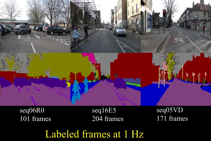
Finally, let's talk about segmentation. This is from the famous CamVid (Cambridge-driving Labeled Video Database) dataset which is a classic example of an academic segmentation dataset. Basically you can see what we do is we start with a picture (they are actually video frames in this dataset) and we have some labels where they are not actually colors — each one has an ID and the IDs are mapped to colors. So red might be 1, purple might be 2, light pink might be 3 and so all the buildings are one class, all the cars are another class, all the people are another class, all the road is another class, and so on. So what we are actually doing here is multi-class classification for every pixel. You can see, sometimes that multi-class classification really is quite tricky — like these branches. Although, sometimes the labels are really not that great. This is very coarse as you can see. So that's what we are going to do.

We are going to do segmentation and so it's a lot like bounding boxes. But rather than just finding a box around each thing, we are actually going to label every single pixel with its class. Really, it's actually a lot easier because it fits our CNN style so nicely that we can create any CNN where the output is an N by M grid containing the integers from 0 to C where there are C categories. And then we can use cross-entropy loss with a softmax activation and we are done. I could actually stop the class there and you can go and use exactly the same approaches you've learnt in lesson 1 and 2 and you'll get a perfectly okay result. So the first thing to say is this is not actually a terribly hard thing to do. But we are going to try and do it really well.

Doing it the simple way [01:31:26]

Notebook

Let's start by doing it the really simple way. And we are going to use Kaggle Carvana competition and you can download it with Kaggle API as usual.

%matplotlib inline
%reload_ext autoreload
%autoreload 2

from fastai.conv_learner import *
from fastai.dataset import *

from pathlib import Path
import json

Setup

There is a train folder containing bunch of images which is the independent variable and a train_masks folder there's the dependent variable and they look like below.

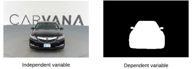
In this case, just like cats and dogs, we are going simple rather than doing multi-class classification, we are going to do binary classification. But of course multi-class is just the more general version — categorical cross entropy or binary class entropy. There is no differences conceptually, so the dependent variable is just zeros and ones, where else the independent variable is a regular image.

In order to do this well, it would really help to know what cars look like. Because really what we want to do is to figure out this is a car and its orientation and put white pixels where we expect the car to be based on the picture and their understanding of what cars look like.

PATH = Path('data/carvana')
list(PATH.iterdir())

# -----------------------------------------------------------------------------
# Output
# -----------------------------------------------------------------------------
[PosixPath('data/carvana/train_masks'),
 PosixPath('data/carvana/train_masks.csv'),
 PosixPath('data/carvana/sample_submission.csv'),
 PosixPath('data/carvana/train'),
 PosixPath('data/carvana/metadata.csv')]

MASKS_FN = 'train_masks.csv'
META_FN = 'metadata.csv'
TRAIN_DN = 'train'
MASKS_DN = 'train_masks'

masks_csv = pd.read_csv(PATH / MASKS_FN)
masks_csv.head()

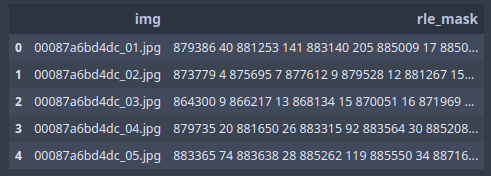
The original dataset came with these CSV files as well [1:32:44]. I don't really use them for very much other than getting the list of images from them.

meta_csv = pd.read_csv(PATH / META_FN)
meta_csv.head()

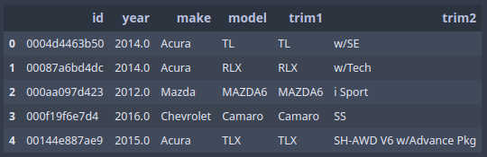
def show_img(im, figsize=None, ax=None, alpha=None):
    if not ax: fig, ax = plt.subplots(figsize=figsize)
    ax.imshow(im, alpha=alpha)
    ax.set_axis_off()
    return ax

CAR_ID = '00087a6bd4dc'

list((PATH / TRAIN_DN).iterdir())[:5]

# -----------------------------------------------------------------------------
# Output
# -----------------------------------------------------------------------------
[PosixPath('data/carvana/train/33a310ea7462_08.jpg'),
 PosixPath('data/carvana/train/f3eee6348205_15.jpg'),
 PosixPath('data/carvana/train/9d8c465a0881_02.jpg'),
 PosixPath('data/carvana/train/c87688f6960e_02.jpg'),
 PosixPath('data/carvana/train/08a646be6b30_07.jpg')]

Image.open(PATH / TRAIN_DN / f'{CAR_ID}_01.jpg').resize((300, 200))

list((PATH / MASKS_DN).iterdir())[:5]

# -----------------------------------------------------------------------------
# Output
# -----------------------------------------------------------------------------
[PosixPath('data/carvana/train_masks/843763f47895_01_mask.gif'),
 PosixPath('data/carvana/train_masks/34b0c08544a5_09_mask.gif'),
 PosixPath('data/carvana/train_masks/8b4b87ad7be6_16_mask.gif'),
 PosixPath('data/carvana/train_masks/61060ada97c9_03_mask.gif'),
 PosixPath('data/carvana/train_masks/5df60cf7cab2_16_mask.gif')]

Image.open(PATH / MASKS_DN / f'{CAR_ID}_01_mask.gif').resize((300, 200))

Each image after the car ID has a 01, 02, etc of which I've printed out all 16 of them for one car and as you can see basically those numbers are the 16 orientations of one car [1:32:58]. I don't think anybody in this competition actually used these orientation information. I believe they all kept the car's images just treated them separately.

ims = [open_image(PATH / TRAIN_DN / f'{CAR_ID}_{i+1:02d}.jpg') for i in range(16)]

fig, axes = plt.subplots(4, 4, figsize=(9, 6))
for i, ax in enumerate(axes.flat):
    show_img(ims[i], ax=ax)
plt.tight_layout(pad=0.1)

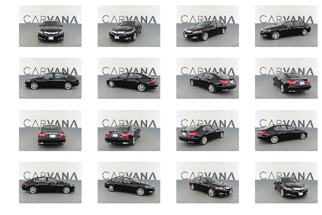
Resize and convert [01:33:27]

These images are pretty big — over 1000 by 1000 in size and just opening the JPEGs and resizing them is slow. So I processed them all. Also OpenCV can't handle GIF files so I converted them.

❓ How would somebody get these masks for training initially? Mechanical Turk or something [1:33:48]?

Yeah, just a lot of boring work. Probably there are some tools that help you with a bit of edge snapping so that the human can do it roughly and then just fine tune the bits it gets wrong. These kinds of labels are expensive. 🔖 So one of the things I really want to work on is deep learning enhanced interactive labeling tools because that's clearly something that would help a lot of people.

I've got a little section here that you can run if you want to. You probably want to. It converts the GIFs into PNGs so just open it up with PIL and then save it as PNG because OpenCV doesn't have GIF support. As per usual for this kind of stuff, I do it with a ThreadPool so I can take advantage of parallel processing. And then also create a separate directory train-128 and train_masks-128 which contains the 128 by 128 resized versions of them.

This is the kind of stuff that keeps you sane if you do it early in the process. So anytime you get a new dataset, seriously think about creating a smaller version to make life fast. Anytime you find yourself waiting on your computer, try and think of a way to create a smaller version.

(PATH / 'train_masks_png').mkdir(exist_ok=True)

def convert_img(fn):
    fn = fn.name
    Image.open(PATH / 'train_masks' / fn).save(PATH / 'train_masks_png' / f'{fn[:-4]}.png')

files = list((PATH / 'train_masks').iterdir())
with ThreadPoolExecutor(8) as e:
    e.map(convert_img, files)

(PATH / 'train_masks-128').mkdir(exist_ok=True)

def resize_mask(fn):
    Image.open(fn).resize((128, 128)).save((fn.parent.parent) / 'train_masks-128' / fn.name)

%%time
files = list((PATH / 'train_masks_png').iterdir())
with ThreadPoolExecutor(8) as e:
    e.map(resize_mask, files)

# -----------------------------------------------------------------------------
# Output
# -----------------------------------------------------------------------------
CPU times: user 32.3 s, sys: 608 ms, total: 32.9 s
Wall time: 8.87 s

(PATH / 'train-128').mkdir(exist_ok=True)

def resize_img(fn):
    Image.open(fn).resize((128, 128)).save((fn.parent.parent) / 'train-128' / fn.name)

%%time
files = list((PATH / 'train').iterdir())
with ThreadPoolExecutor(8) as e:
    e.map(resize_img, files)

# -----------------------------------------------------------------------------
# Output
# -----------------------------------------------------------------------------
CPU times: user 4min 2s, sys: 640 ms, total: 4min 3s
Wall time: 1min 2s

So after you grab it from Kaggle, you probably want to run this stuff, go away, have lunch, come back and when you are done, you'll have these smaller directories which we are going to use below 128 by 128 to start with.

Dataset [01:35:33]

TRAIN_DN = 'train-128'
MASKS_DN = 'train_masks-128'
sz = 128
bs = 64

ims = [open_image(PATH / TRAIN_DN / f'{CAR_ID}_{i+1:02d}.jpg') for i in range(16)]
im_masks = [open_image(PATH / MASKS_DN / f'{CAR_ID}_{i+1:02d}_mask.png') for i in range(16)]

So here is a cool trick. If you use the same axis object (ax) to plot an image twice and the second time you use alpha which you might know means transparency in the computer vision world, then you can actually plot the mask over the top of the photo. So here is a nice way to see all the masks on top of the photos for all of the cars in one group.

fig, axes = plt.subplots(4, 4, figsize=(12, 10))
for i, ax in enumerate(axes.flat):
    ax = show_img(ims[i], ax=ax)
    show_img(im_masks[i][..., 0], ax=ax, alpha=0.5)
plt.tight_layout(pad=0.1)

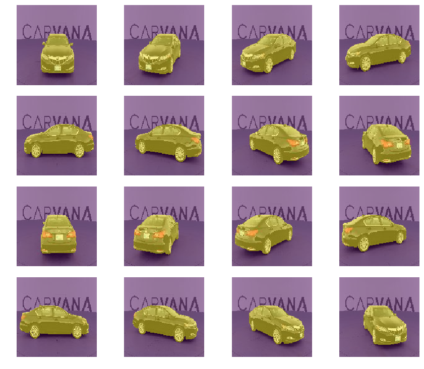
This is the same MatchedFilesDataset we've seen twice already. This is all the same code. Here is something important though. If we had something that was in the training set the one on the left, and then the validation had the image on the right, that would be kind of cheating because it's the same car.

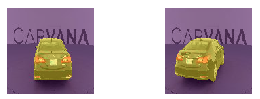
class MatchedFilesDataset(FilesDataset):
    def __init__(self, fnames, y, transform, path):
        self.y = y
        assert(len(fnames) == len(y))
        super().__init__(fnames, transform, path)

    def get_y(self, i): return open_image(os.path.join(self.path, self.y[i]))

    def get_c(self): return 0

x_names = np.array([Path(TRAIN_DN) / o for o in masks_csv['img']])
y_names = np.array([Path(MASKS_DN) / f'{o[:-4]}_mask.png' for o in masks_csv['img']])

len(x_names) // 16 // 5 * 16

# -----------------------------------------------------------------------------
# Output
# -----------------------------------------------------------------------------
1008

So we use a continuous set of car IDs and since each set is a set of 16, we make sure that's evenly divisible by 16. So we make sure that our validation set contains different car IDs to our training set. This is the kind of stuff which you've got to be careful of. On Kaggle, it's not so bad — you'll know about it because you'll submit your result and you'll get a very different result on your leaderboard compared to your validation set. But in the real world. you won't know until you put it in production and send your company bankrupt and lose your job. So you might want to think carefully about your validation set in that case.

val_idxs = list(range(1008))
((val_x, trn_x), (val_y, trn_y)) = split_by_idx(val_idxs, x_names, y_names)
len(val_x), len(trn_x)

# -----------------------------------------------------------------------------
# Output
# -----------------------------------------------------------------------------
(1008, 4080)

Here we are going to use transform type classification (TfmType.CLASS) [1:37:03]. It's basically the same as transform type pixel (TfmType.PIXEL) but if you think about it, with a pixel version if we rotate a little bit then we probably want to average the pixels in between the two, but the classification, obviously we don't. We use nearest neighbor. So there's slight difference there. Also for classification, lighting doesn't kick in, normalization doesn't kick in to the dependent variable.

aug_tfms = [RandomRotate(4, tfm_y=TfmType.CLASS),
            RandomFlip(tfm_y=TfmType.CLASS),
            RandomLighting(0.05, 0.05)]
# aug_tfms = []

They are already square images, so we don't have to do any cropping.

tfms = tfms_from_model(resnet34, sz, crop_type=CropType.NO, tfm_y=TfmType.CLASS, aug_tfms=aug_tfms)
datasets = ImageData.get_ds(MatchedFilesDataset, (trn_x, trn_y), (val_x, val_y), tfms, path=PATH)
md = ImageData(PATH, datasets, bs, num_workers=8, classes=None)

denorm = md.trn_ds.denorm
x, y = next(iter(md.aug_dl))
x = denorm(x)

So here you can see different versions of the augmented images — they are moving around a bit, and they are rotating a bit, and so forth.

fig, axes = plt.subplots(5, 6, figsize=(12, 10))
for i, ax in enumerate(axes.flat):
    ax = show_img(x[i], ax=ax)
    show_img(y[i], ax=ax, alpha=0.5)
plt.tight_layout(pad=0.1)

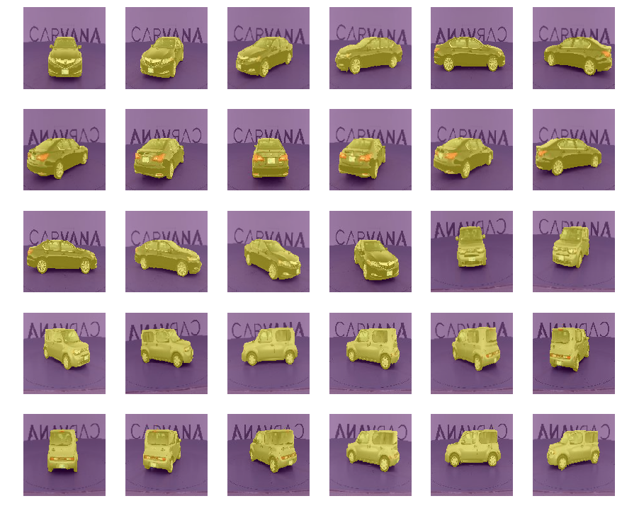
I get a lot of questions during our study group about how do I debug things and fix things that aren't working. I never have a great answer other than every time I fix a problem is because of stuff like this that I do all the time. I just always print out everything as I go and then the one thing that I screw up always turns out to be the one thing that I forgot to check along the way. The more of this kind of thing you can do, the better. If you are not looking at all of your intermediate results, you are going to have troubles.

Model [01:38:30]

class Empty(nn.Module):
    def forward(self, x): return x

models = ConvnetBuilder(resnet34, 0, 0, 0, custom_head=Empty())
learn = ConvLearner(md, models)
learn.summary()

class StdUpsample(nn.Module):
    def __init__(self, nin, nout):
        super().__init__()
        self.conv = nn.ConvTranspose2d(nin, nout, 2, stride=2)
        self.bn = nn.BatchNorm2d(nout)

    def forward(self, x): return self.bn(F.relu(self.conv(x)))

flatten_channel = Lambda(lambda x: x[:, 0])

simple_up = nn.Sequential(
    nn.ReLU(),
    StdUpsample(512, 256),
    StdUpsample(256, 256),
    StdUpsample(256, 256),
    StdUpsample(256, 256),
    nn.ConvTranspose2d(256, 1, 2, stride=2),
    flatten_channel
)

Given that we want something that knows what cars look like, we probably want to start with a pre-trained ImageNet network. So we are going to start with ResNet34. With ConvnetBuilder, we can grab our ResNet34 and we can add a custom head. The custom head is going to be something that upsamples a bunch of times and we are going to do things really dumb for now which is we're just going to do a ConvTranspose2d, batch norm, ReLU.

This is what I am saying — any of you could have built this without looking at any of this notebook or at least you have the information from previous classes. There is nothing new at all. So at the very end, we have a single filter. Now that's going to give us something which is batch size by 1 by 128 by 128. But we want something which is batch size by 128 by 128. So we have to remove that unit axis so I've got a lambda layer here. Lambda layers are incredibly helpful because without the lambda layer here, which is simply removing that unit axis by just indexing it with a 0, without a lambda layer, I would have to have created a custom class with a custom forward method and so forth. But by creating a lambda layer that does the one custom bit, I can now just chuck it in the Sequential and so that makes life easier.

PyTorch people are kind of snooty about this approach. Lambda layer is actually something that's a part of the fastai library not part of the PyTorch library. And literally people on PyTorch discussion board say "yes, we could give people this", "yes it is only a single line of code" but they never encourage them to use sequential too often. So there you go.

So this is our custom head [1:40:36]. So we are going to have a ResNet 34 that goes downsample and then a really simple custom head that very quickly upsamples, and that hopefully will do something. And we are going to use accuracy with a threshold of 0.5 and print out metrics.

models = ConvnetBuilder(resnet34, 0, 0, 0, custom_head=simple_up)
learn = ConvLearner(md, models)
learn.opt_fn = optim.Adam
learn.crit = nn.BCEWithLogitsLoss()
learn.metrics = [accuracy_thresh(0.5)]

learn.lr_find()
learn.sched.plot()

# -----------------------------------------------------------------------------
# Output
# -----------------------------------------------------------------------------
86%|████████▌ | 55/64 [00:17<00:02,  3.19it/s, loss=2.57]

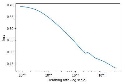
lr = 4e-2

%time learn.fit(lr, 1, cycle_len=5, use_clr=(20, 5))

# -----------------------------------------------------------------------------
# Output
# -----------------------------------------------------------------------------
epoch      trn_loss   val_loss   <lambda>
    0      0.178128   0.133835   0.943451
    1      0.127164   0.116731   0.947308
    2      0.106335   0.104343   0.956882
    3      0.095134   0.095054   0.9587
    4      0.087233   0.089795   0.961317
[array([0.0898]), 0.9613169706056989]

CPU times: user 2min 24s, sys: 31.2 s, total: 2min 56s
Wall time: 2min 11s

After a few epochs, we've got 96 percent accurate. Is that good [1:40:56]? Is 96% accurate good? And hopefully the answer to that question is it depends. What's it for? The answer is Carvana wanted this because they wanted to be able to take their car image and cut them out and paste them on exotic Monte Carlo backgrounds or whatever (that's Monte Carlo the place and not the simulation). To do that, you you need a really good mask. You don't want to leave the rearview mirrors behind, have one wheel missing, or include a little bit of background or something. That would look stupid. So you would need something very good. So only having 96% of the pixels correct doesn't sound great. But we won't really know until we look at it. So let's look at it.

learn.save('tmp')

learn.load('tmp')

py,ay = learn.predict_with_targs()

ay.shape

# -----------------------------------------------------------------------------
# Output
# -----------------------------------------------------------------------------
(1008, 128, 128)

So there is the correct version that we want to cut out [1:41:54].

show_img(ay[0])

That's the 96% accurate version. So when you look at it you realize "oh yeah, getting 96% of the pixel accurate is actually easy because all the outside bit is not car, and all the inside bit is a car, and really interesting bit is the edge. So we need to do better.

show_img(py[0] > 0)

Let's unfreeze because all we've done so far is train the custom head. Let's do more.

learn.unfreeze()

learn.bn_freeze(True)

lrs = np.array([lr / 100, lr / 10, lr]) / 4

%time learn.fit(lrs, 1, cycle_len=20, use_clr=(20, 10))

# -----------------------------------------------------------------------------
# Output
# -----------------------------------------------------------------------------
epoch      trn_loss   val_loss   mask_acc
    0      0.015785   0.020673   0.99169
    1      0.017603   0.022358   0.990212
    2      0.018592   0.022732   0.99128
    3      0.019646   0.023073   0.990465
    4      0.018345   0.021401   0.990871
    5      0.017203   0.020322   0.991719
    6      0.016402   0.020434   0.991706
    7      0.015707   0.02045    0.991949
    8      0.01529    0.019834   0.992149
    9      0.014755   0.019734   0.992234
    10     0.014321   0.019756   0.99238
    11     0.013958   0.019861   0.992505
    12     0.013527   0.019761   0.992431
    13     0.013237   0.019764   0.99273
    14     0.012983   0.019742   0.992547
    15     0.012557   0.019709   0.992447
    16     0.012256   0.019784   0.992856
    17     0.01197    0.019746   0.992907
    18     0.011691   0.019741   0.993008
    19     0.01147    0.019642   0.993041
[array([0.01964]), 0.9930412665246025]

CPU times: user 16min 26s, sys: 2min 20s, total: 18min 46s
Wall time: 15min

After a bit more, we've got 99.1%. Is that good? I don't know. Let's take a look.

learn.save('0')

x, y = next(iter(md.val_dl))
py = to_np(learn.model(V(x)))

Actually no. It's totally missed the rearview vision mirror on the left and missed a lot of it on the right. And it's clearly got an edge wrong on the bottom. And these things are totally going to matter when we try to cut it out, so it's still not good enough.

ax = show_img(denorm(x)[0])
show_img(py[0] > 0, ax=ax, alpha=0.5)

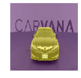
ax = show_img(denorm(x)[0])
show_img(y[0], ax=ax, alpha=0.5)

512x512 [01:42:50]

Let's try upscaling. And the nice thing is that when we upscale to 512 by 512, (make sure you decrease the batch size because you'll run out of memory), it's quite a lot more information there for it to go on so our accuracy increases to 99.4% and things keep getting better.

TRAIN_DN = 'train'
MASKS_DN = 'train_masks_png'
sz = 512
bs = 16

x_names = np.array([Path(TRAIN_DN) / o for o in masks_csv['img']])
y_names = np.array([Path(MASKS_DN) / f'{o[:-4]}_mask.png' for o in masks_csv['img']])

((val_x, trn_x), (val_y, trn_y)) = split_by_idx(val_idxs, x_names, y_names)
len(val_x), len(trn_x)

# -----------------------------------------------------------------------------
# Output
# -----------------------------------------------------------------------------
(1008, 4080)

tfms = tfms_from_model(resnet34, sz, crop_type=CropType.NO, tfm_y=TfmType.CLASS, aug_tfms=aug_tfms)
datasets = ImageData.get_ds(MatchedFilesDataset, (trn_x, trn_y), (val_x, val_y), tfms, path=PATH)
md = ImageData(PATH, datasets, bs, num_workers=8, classes=None)

denorm = md.trn_ds.denorm
x, y = next(iter(md.aug_dl))
x = denorm(x)

Here is the true ones.

fig, axes = plt.subplots(4, 4, figsize=(10, 10))
for i, ax in enumerate(axes.flat):
    ax = show_img(x[i], ax=ax)
    show_img(y[i], ax=ax, alpha=0.5)
plt.tight_layout(pad=0.1)

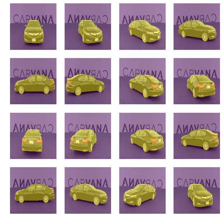
simple_up = nn.Sequential(
    nn.ReLU(),
    StdUpsample(512, 256),
    StdUpsample(256, 256),
    StdUpsample(256, 256),
    StdUpsample(256, 256),
    nn.ConvTranspose2d(256, 1, 2, stride=2),
    flatten_channel
)

models = ConvnetBuilder(resnet34, 0, 0, 0, custom_head=simple_up)
learn = ConvLearner(md, models)
learn.opt_fn = optim.Adam
learn.crit = nn.BCEWithLogitsLoss()
learn.metrics = [accuracy_thresh(0.5)]

learn.load('0')

learn.lr_find()
learn.sched.plot()

# -----------------------------------------------------------------------------
# Output
# -----------------------------------------------------------------------------
80%|███████▉  | 203/255 [04:16<01:05,  1.26s/it, loss=0.901]

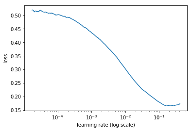
lr = 4e-2

%time learn.fit(lr, 1, cycle_len=5, use_clr=(20, 5))

# -----------------------------------------------------------------------------
# Output
# -----------------------------------------------------------------------------
Epoch 100% 5/5 [31:15<00:00, 375.10s/it]

epoch      trn_loss   val_loss   mask_acc
    0      0.053045   0.056443   0.976122
    1      0.034384   0.03848    0.982819
    2      0.029025   0.028036   0.98826
    3      0.025769   0.026095   0.990837
    4      0.023503   0.023225   0.99101
[array([0.02322]), 0.9910101739187089]

CPU times: user 1h 17min 27s, sys: 7min 36s, total: 1h 25min 3s
Wall time: 31min 16s

learn.save('tmp')

learn.load('tmp')

learn.unfreeze()
learn.bn_freeze(True)

lrs = np.array([lr / 100, lr / 10, lr]) / 4

%time learn.fit(lrs, 1, cycle_len=8, use_clr=(20, 8))

# -----------------------------------------------------------------------------
# Output
# -----------------------------------------------------------------------------
Epoch 100% 8/8 [1:27:53<00:00, 659.16s/it]

epoch      trn_loss   val_loss   mask_acc
    0      0.016866   0.012258   0.995355
    1      0.009588   0.009799   0.995858
    2      0.008489   0.009014   0.996504
    3      0.00801    0.008541   0.996556
    4      0.007585   0.008287   0.996624
    5      0.007114   0.008004   0.996836
    6      0.007005   0.007713   0.996924
    7      0.006721   0.007581   0.996972
[array([0.00758]), 0.9969720689077226]

CPU times: user 2h 40min 40s, sys: 12min 6s, total: 2h 52min 46s
Wall time: 1h 27min 54s

learn.save('512')

x, y = next(iter(md.val_dl))
py = to_np(learn.model(V(x)))

ax = show_img(denorm(x)[0])
show_img(py[0] > 0, ax=ax, alpha=0.5)

ax = show_img(denorm(x)[0])
show_img(y[0], ax=ax, alpha=0.5)

Things keep getting better but we've still got quite a few little black blocky bits. so let's go to 1024 by 1024.

1024x1024 [01:43:17]

So let's go to 1024 by 1024, batch size down to 4. This is pretty high res now, and train a bit more, 99.6, 99.8%!

sz = 1024
bs = 4

tfms = tfms_from_model(resnet34, sz, crop_type=CropType.NO, tfm_y=TfmType.CLASS, aug_tfms=aug_tfms)
datasets = ImageData.get_ds(MatchedFilesDataset, (trn_x, trn_y), (val_x, val_y), tfms, path=PATH)
md = ImageData(PATH, datasets, bs, num_workers=8, classes=None)

denorm = md.trn_ds.denorm
x, y = next(iter(md.aug_dl))
x = denorm(x)
y = to_np(y)

fig, axes = plt.subplots(2, 2, figsize=(8, 8))
for i, ax in enumerate(axes.flat):
    show_img(x[i], ax=ax)
    show_img(y[i], ax=ax, alpha=0.5)
plt.tight_layout(pad=0.1)

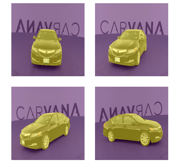
simple_up = nn.Sequential(
    nn.ReLU(),
    StdUpsample(512, 256),
    StdUpsample(256, 256),
    StdUpsample(256, 256),
    StdUpsample(256, 256),
    nn.ConvTranspose2d(256, 1, 2, stride=2),
    flatten_channel,
)

models = ConvnetBuilder(resnet34, 0, 0, 0, custom_head=simple_up)
learn = ConvLearner(md, models)
learn.opt_fn = optim.Adam
learn.crit = nn.BCEWithLogitsLoss()
learn.metrics = [accuracy_thresh(0.5)]

learn.load('512')

%%time
learn.lr_find()
learn.sched.plot()

# -----------------------------------------------------------------------------
# Output
# -----------------------------------------------------------------------------
70%|███████   | 717/1020 [13:42<05:47,  1.15s/it, loss=0.0861]

CPU times: user 22min 29s, sys: 2min 50s, total: 25min 20s
Wall time: 13min 42s

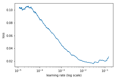
lr = 4e-2

learn.fit(lr, 1, cycle_len=2, use_clr=(20, 4))

# -----------------------------------------------------------------------------
# Output
# -----------------------------------------------------------------------------
Epoch 100% 2/2 [45:21<00:00, 1360.98s/it]

epoch      trn_loss   val_loss   mask_acc
    0      0.010187   0.010713   0.996185
    1      0.0086     0.008232   0.997017
[array([0.00823]), 0.9970168187504723]

learn.save('tmp')

learn.load('tmp')

learn.unfreeze()
learn.bn_freeze(True)

lrs = np.array([lr / 100, lr / 10, lr]) / 8

learn.fit(lrs, 1, cycle_len=40, use_clr=(20, 10))

# -----------------------------------------------------------------------------
# Output
# -----------------------------------------------------------------------------
epoch      trn_loss   val_loss   mask_acc
    0      0.005643   0.006067   0.997681
    1      0.0054     0.006054   0.997656
    2      0.005204   0.005574   0.997634
    3      0.005528   0.00666    0.997664
    4      0.006686   0.007286   0.997451
    5      0.006337   0.006863   0.997468
    6      0.005324   0.006193   0.997629
    7      0.005142   0.005845   0.997886
    8      0.005111   0.005904   0.997774
    9      0.005092   0.005472   0.997967
    10     0.004898   0.005497   0.997801
    11     0.010694   0.007598   0.997152
    12     0.004787   0.005513   0.997856
    13     0.004599   0.005142   0.997935
    14     0.004655   0.005915   0.997716
    15     0.004294   0.005211   0.998055
[0.0052112686, 0.99805523208291195]

It took me ~37 minutes (2195.4s) to train 1 epoch on a K80 GPU, roughly 1.99s/iteration. The GPU memory usage peak at ~10 GB. The full training should take me like 25 hours. So it's kind of slow. I stop training after epoch 15 and that took like 10 hours.

learn.save('1024-cyc-len-40-clr-20-10-epoch-15')

x, y = next(iter(md.val_dl))
py = to_np(learn.model(V(x)))

ax = show_img(denorm(x)[0])
show_img(py[0][0] > 0, ax=ax, alpha=0.5)

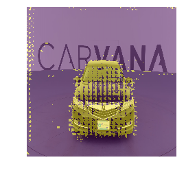
ax = show_img(denorm(x)[0])
show_img(y[0, ..., -1], ax=ax, alpha=0.5)

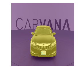
show_img(py[0][0] > 0)

show_img(y[0, ..., -1])

Things not getting better. So, let's resume training from the point where we stop previously at epoch 15. An epoch took me ~27 minutes this time when I have set torch.backends.cudnn.benchmark to True. Save around 10 minutes per epoch.

%time learn.fit(lrs, 1, cycle_len=25, use_clr=(20, 10))

# -----------------------------------------------------------------------------
# Output
# -----------------------------------------------------------------------------
Epoch 100% 25/25 [12:12:00<00:00, 1756.82s/it]

epoch      trn_loss   val_loss   mask_acc
    0      0.004155   0.004891   0.998142
    1      0.005067   0.005655   0.997962
    2      0.005128   0.005889   0.997714
    3      0.00461    0.005717   0.99765
    4      0.004372   0.00531    0.998056
    5      0.004275   0.004979   0.998043
    6      0.004037   0.004815   0.998145
    7      0.003934   0.004865   0.997999
    8      0.004223   0.00502    0.998106
    9      0.00415    0.004842   0.998115
    10     0.003837   0.0047     0.998175
    11     0.004021   0.004518   0.998168
    12     0.003821   0.004748   0.998147
    13     0.003632   0.004656   0.998237
    14     0.003683   0.004457   0.998251
    15     0.003567   0.004629   0.998135
    16     0.003487   0.004385   0.998262
    17     0.003454   0.004546   0.99824
    18     0.003489   0.004387   0.998334
    19     0.003503   0.004257   0.998329
    20     0.003333   0.004442   0.998278
    21     0.003314   0.004375   0.998324
    22     0.003169   0.00438    0.998337
    23     0.003208   0.004365   0.998367
    24     0.003272   0.004338   0.998363
[array([0.00434]), 0.9983625430909414]
CPU times: user 18h 41min 28s, sys: 1h 31min 20s, total: 20h 12min 48s
Wall time: 12h 12min 2s

learn.save('1024-cyc-len-25-clr-20-10')

x, y = next(iter(md.val_dl))
py = to_np(learn.model(V(x)))

After 25 epochs, we've got 99.8 percent accurate.

Plot the mask over the top of the photo.

ax = show_img(denorm(x)[0])
show_img(py[0] > 0, ax=ax, alpha=0.5)

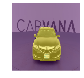
ax = show_img(denorm(x)[0])
show_img(y[0], ax=ax, alpha=0.5)

Plot just the mask.

show_img(py[0] > 0)

show_img(y[0])

Now if we look at the masks, they are actually looking not bad. That's looking pretty good. So can we do better? And the answer is yes, we can.

U-Net [01:43:45]

• Notebook
• Paper

U-Net network is quite magnificent. With that previous approach, our pre-trained ImageNet network was being squished down all the way down to 7x7 and then expand it out all the way back up to 224x224 (1024 gets squished down to quite a bit bigger than 7x7). And then expanded out again all this way which means it has to somehow store all the information about the much bigger version in the small version. And actually most of the information about the bigger version was really in the original picture anyway. So it doesn't seem like a great approach — this squishing and un-squishing.

So the U-Net idea comes from this fantastic paper where it was literally invented in this very domain-specific area of biomedical image segmentation. But in fact, basically every Kaggle winner in anything even vaguely related to segmentation has end up using U-Net. It's one of these things that everybody in Kaggle knows it is the best practice, but in more of academic circles, this has been around for a couple of years at least, a lot of people still don't realize this is by far the best approach.

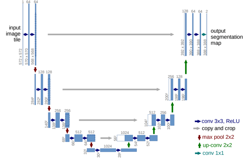
Here is the basic idea [1:45:10]. On the left is the downward path where we start at 572x572 in this case then halve the grid size 4 times, then on the right is the upward path where we double the grid size 4 times. But the thing that we also do is, at every point where we halve the grid size, we actually copy those activations over to the upward path and concatenate them together.

You can see on the bottom right, these red arrows are max pooling operation, these green arrows are upward sampling, and then these gray arrows are copying. So we copy and concat. In other words, the input image after a couple of convs is copied over to the output, concatenated together, and so now we get to use all of the informations gone through all the down and all the up, plus also a slightly modified version of the input pixels. And slightly modified version of one thing down from the input pixels because they came up through here. So we have all of the richness of going all the way down and up, but also a slightly less coarse version and a slightly less coarse version and then the really simple version, and they can all be combined together. So that's U-Net. It's such a cool idea.

Here we are in the carvana-unet notebook. All this is the same code as before.

%matplotlib inline
%reload_ext autoreload
%autoreload 2

from fastai.conv_learner import *
from fastai.dataset import *
from fastai.models.resnet import vgg_resnet50

import json
torch.backends.cudnn.benchmark = True

Data

PATH = Path('data/carvana')
MASKS_FN = 'train_masks.csv'
META_FN = 'metadata.csv'
masks_csv = pd.read_csv(PATH / MASKS_FN)
meta_csv = pd.read_csv(PATH / META_FN)

def show_img(im, figsize=None, ax=None, alpha=None):
    if not ax: fig, ax = plt.subplots(figsize=figsize)
    ax.imshow(im, alpha=alpha)
    ax.set_axis_off()
    return ax

TRAIN_DN = 'train-128'
MASKS_DN = 'train_masks-128'
sz = 128
bs = 64
nw = 16

TRAIN_DN = 'train'
MASKS_DN = 'train_masks_png'
sz = 128
bs = 64
nw = 16

class MatchedFilesDataset(FilesDataset):
    def __init__(self, fnames, y, transform, path):
        self.y = y
        assert(len(fnames) == len(y))
        super().__init__(fnames, transform, path)

    def get_y(self, i): return open_image(os.path.join(self.path, self.y[i]))

    def get_c(self): return 0

x_names = np.array([Path(TRAIN_DN) / o for o in masks_csv['img']])
y_names = np.array([Path(MASKS_DN) / f'{o[:-4]}_mask.png' for o in masks_csv['img']])

val_idxs = list(range(1008))
((val_x, trn_x), (val_y, trn_y)) = split_by_idx(val_idxs, x_names, y_names)

aug_tfms = [RandomRotate(4, tfm_y=TfmType.CLASS),
            RandomFlip(tfm_y=TfmType.CLASS),
            RandomLighting(0.05, 0.05, tfm_y=TfmType.CLASS)]

tfms = tfms_from_model(resnet34, sz, crop_type=CropType.NO, tfm_y=TfmType.CLASS, aug_tfms=aug_tfms)
datasets = ImageData.get_ds(MatchedFilesDataset, (trn_x, trn_y), (val_x, val_y), tfms, path=PATH)
md = ImageData(PATH, datasets, bs, num_workers=16, classes=None)
denorm = md.trn_ds.denorm

x, y = next(iter(md.trn_dl))

x.shape, y.shape

# -----------------------------------------------------------------------------
# Output
# -----------------------------------------------------------------------------
(torch.Size([64, 3, 128, 128]), torch.Size([64, 128, 128]))

Simple upsample

And at the start, I've got a simple upsample version just to show you again the non U-net version. This time, I'm going to add in something called the dice metric. Dice is very similar, as you see, to Jaccard or I over U. It's just a minor difference. It's basically intersection over union with a minor tweak. The reason we are going to use dice is that's the metric that Kaggle competition used and it's a little bit harder to get a high dice score than a high accuracy because it's really looking at what the overlap of the correct pixels are with your pixels. But it's pretty similar.

So in the Kaggle competition, people that were doing okay were getting about 99.6 dice and the winners were about 99.7 dice.

f = resnet34
cut, lr_cut = model_meta[f]

def get_base():
    layers = cut_model(f(True), cut)
    return nn.Sequential(*layers)

def dice(pred, targs):
    pred = (pred > 0).float()
    return 2. * (pred * targs).sum() / (pred + targs).sum()

Here is our standard upsample.

class StdUpsample(nn.Module):
    def __init__(self, nin, nout):
        super().__init__()
        self.conv = nn.ConvTranspose2d(nin, nout, 2, stride=2)
        self.bn = nn.BatchNorm2d(nout)

    def forward(self, x): return self.bn(F.relu(self.conv(x)))

This all as before.

class Upsample34(nn.Module):
    def __init__(self, rn):
        super().__init__()
        self.rn = rn # resnet
        self.features = nn.Sequential(
            rn, nn.ReLU(),
            StdUpsample(512, 256),
            StdUpsample(256, 256),
            StdUpsample(256, 256),
            StdUpsample(256, 256),
            nn.ConvTranspose2d(256, 1, 2, stride=2))

    def forward(self, x): return self.features(x)[:, 0]

class UpsampleModel():
    def __init__(self, model, name='upsample'):
        self.model, self.name = model, name

    def get_layer_groups(self, precompute):
        lgs = list(split_by_idxs(children(self.model.rn), [lr_cut]))
        return lgs + [children(self.model.features)[1:]]

m_base = get_base()

m = to_gpu(Upsample34(m_base))
models = UpsampleModel(m)

learn = ConvLearner(md, models)
learn.opt_fn = optim.Adam
learn.crit = nn.BCEWithLogitsLoss()
learn.metrics = [accuracy_thresh(0.5), dice]

learn.freeze_to(1)

learn.lr_find()
learn.sched.plot()

# -----------------------------------------------------------------------------
# Output
# -----------------------------------------------------------------------------
84%|████████▍ | 54/64 [00:19<00:03,  2.70it/s, loss=2.81]

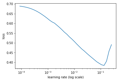
lr = 4e-2
wd = 1e-7
lrs = np.array([lr / 100, lr / 10, lr]) / 2

%time learn.fit(lr, 1, wds=wd, cycle_len=4, use_clr=(20, 8))

# -----------------------------------------------------------------------------
# Output
# -----------------------------------------------------------------------------
Epoch 100% 4/4 [01:38<00:00, 24.63s/it]

epoch      trn_loss   val_loss   <lambda>   dice
    0      0.115094   0.052829   0.977156   0.946632
    1      0.060572   0.041022   0.981844   0.958449
    2      0.041211   0.037313   0.981443   0.960839
    3      0.033257   0.029371   0.986961   0.971081
[array([0.02937]), 0.9869610014415923, 0.9710806340169884]
CPU times: user 2min 1s, sys: 21.1 s, total: 2min 23s
Wall time: 1min 38s

learn.save('tmp')

learn.load('tmp')

learn.unfreeze()
learn.bn_freeze(True)

learn.fit(lrs, 1, cycle_len=4, use_clr=(20, 8))

# -----------------------------------------------------------------------------
# Output
# -----------------------------------------------------------------------------
epoch      trn_loss   val_loss   <lambda>   dice
    0      0.174897   0.061603   0.976321   0.94382
    1      0.122911   0.053625   0.982206   0.957624
    2      0.106837   0.046653   0.985577   0.965792
    3      0.099075   0.042291   0.986519   0.968925
[0.042291240323157536, 0.986519161670927, 0.9689251193924556]

Now we can check our dice metric [1:48:00]. So you can see on dice metric, we are getting around 96.8 at 128x128. So that's not great.

learn.save('128')

x, y = next(iter(md.val_dl))
py = to_np(learn.model(V(x)))

show_img(py[0] > 0)

show_img(y[0])

U-net (ish) [01:48:16]

So let's try U-Net. I'm calling it U-net(ish) because as per usual I'm creating my own somewhat hacky version — trying to keep things as similar to what you're used to as possible and doing things that I think makes sense. So there should be plenty of opportunity for you to at least make this more authentically U-net by looking at the exact grid sizes and see how here (the top left convs) the size is going down a little bit. So they are obviously not adding any padding and then there are some cropping going on — there's a few differences. But one of the things is because I want to take advantage of transfer learning — that means I can't quite use U-Net.

Pre-trained U-Net on ImageNet

🔖 So here is another big opportunity is what if you create the U-Net down path and then add a classifier on the end and then train that on ImageNet. You've now got an ImageNet trained classifier which is specifically designed to be a good backbone for U-Net. Then you should be able to now come back and get pretty closed to winning this old competition (it's actually not that old — it's fairly recent competition). Because that pre-trained network didn't exist before. But if you think about what YOLO v3 did, it's basically that. They created a DarkNet, they pre-trained it on ImageNet, and then they used it as the basis for their bounding boxes. So again, this idea of pre-training things which are designed not just for classification but designed for other things — it's just something that nobody has done yet. But as we've shown, you can train ImageNet for $25 in three hours now. And if people in the community are interested in doing this, hopefully I'll have credits I can help you with as well so if you do, the work to get it set up and give me a script, I can probably run it for you. For now though, we don't have that yet. So we are going to use ResNet.

class SaveFeatures():
    features = None

    def __init__(self, m): self.hook = m.register_forward_hook(self.hook_fn)

    def hook_fn(self, module, input, output): self.features = output

    def remove(self): self.hook.remove()

So we are basically going to start with get_base [1:50:37]. Base is our base network and that was defined back up in the first section.

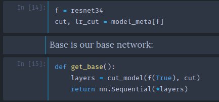
So get_base is going to be something that calls whatever f is and f is resnet34. So we are going to grab our ResNet34 and cut_model is the first thing that our convnet builder does. It basically removes everything from the adaptive pooling onwards, so that gives us back the backbone of ResNet34. So get_base is going to give us back the ResNet34 backbone.

class UnetBlock(nn.Module):
    def __init__(self, up_in, x_in, n_out):
        super().__init__()
        up_out = x_out = n_out // 2
        self.x_conv = nn.Conv2d(x_in, x_out, 1)
        self.tr_conv = nn.ConvTranspose2d(up_in, up_out, 2, stride=2)
        self.bn = nn.BatchNorm2d(n_out)

    def forward(self, up_p, x_p):
        up_p = self.tr_conv(up_p) # up path
        x_p = self.x_conv(x_p) # cross path
        cat_p = torch.cat([up_p, x_p], dim=1) # dim 1 means concat from means left to right
        return self.bn(F.relu(cat_p))

class Unet34(nn.Module):
    def __init__(self, rn):
        super().__init__()
        self.rn = rn # the passed in encoder, example ResNet34
        self.sfs = [SaveFeatures(rn[i]) for i in [2, 4, 5, 6]]
        # calculating connections and channels suck!
        self.up1 = UnetBlock(512, 256, 256)
        self.up2 = UnetBlock(256, 128, 256)
        self.up3 = UnetBlock(256, 64, 256)
        self.up4 = UnetBlock(256, 64, 256)
        self.up5 = nn.ConvTranspose2d(256, 1, 2, stride=2)

    def forward(self, x):
        x = F.relu(self.rn(x))
        x = self.up1(x, self.sfs[3].features)
        x = self.up2(x, self.sfs[2].features)
        x = self.up3(x, self.sfs[1].features)
        x = self.up4(x, self.sfs[0].features)
        x = self.up5(x)
        return x[:, 0]

    def close(self):
        for sf in self.sfs: sf.remove()

class UnetModel():
    def __init__(self, model, name='unet'):
        self.model, self.name = model, name

    def get_layer_groups(self, precompute):
        lgs = list(split_by_idxs(children(self.model.rn), [lr_cut])) # type of lr_cut is int. val is 6
        return lgs + [children(self.model)[1:]]

Then we are going to take that ResNet34 backbone and turn it into a, I call it a, Unet34 [1:51:17]. So what that's going to do is it's going to save that ResNet that we passed in and then we are going to use a forward hook just like before to save the results at the 2nd, 4th, 5th, and 6th blocks which as before is the layers before each stride 2 convolution. Then we are going to create a bunch of these things we are calling UnetBlock. We need to tell UnetBlock how many things are coming from the previous layer we are upsampling, how many are coming across, and then how many do we want to come out. The amount coming across is entirely defined by whatever the base network was — whatever the downward path was, we need that many layers. So this is a little bit awkward. Actually one of our master's students here, Kerem, has actually created something called DynamicUnet that you'll find in fastai.model.DynamicUnet and it actually calculates this all for you and automatically creates the whole U-Net from your base model. It's got some minor quirks still that I want to fix. By the time the video is out, it'll definitely be working and I will at least have a notebook showing how to use it and possibly an additional video. But for now you'll just have to go through and do it yourself. You can easily see it just by, once you've got a ResNet, you can just type in its name and it'll print out the layers. And you can see how many many activations there are in each block. Or you can have it printed out for you for each block automatically. Anyway, I just did this manually.

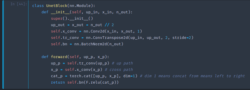
So the UnetBlock works like this [1:53:29]:

• up_in : This many are coming up from the previous layer
• x_in : This many are coming across (hence x) from the downward path
• n_out : The amount we want coming out

Now what I do is, I then say, okay we're going to create a certain amount of convolutions from the upward path and a certain amount from the cross path, and so I'm going to be concatenating them together so let's divide the number we want out by 2. And so we are going to have our cross convolution take our cross path and create number out divided by 2 (n_out//2). And then the upward path is going to be a ConvTranspose2d because we want to increase/upsample. Again here, we've got the number out divided by 2 (up_out), then at the end, I just concatenate those together.

So I've got an upward sample, I've got a cross convolution, I can concatenate the two together. That's all a UnetBlock is. So that's actually a pretty easy module to create.

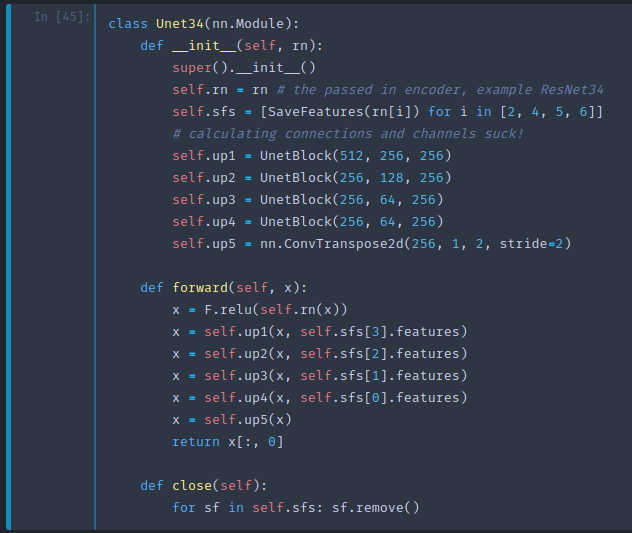
Then in my forward path, I need to pass to the forward of the UnetBlock the upward path and the cross path [1:54:40]. The upward path is just whatever I am up to so far. But then the cross path is whatever the activations are that I stored on the way down. So as I come up, it's the last set of saved features that I need first. And as I gradually keep going up farther and farther, eventually it's the first set of features.

m_base = get_base()
m = to_gpu(Unet34(m_base))
models = UnetModel(m)

learn = ConvLearner(md, models)
learn.opt_fn = optim.Adam
learn.crit=nn.BCEWithLogitsLoss()
learn.metrics=[accuracy_thresh(0.5), dice]

learn.summary()

# -----------------------------------------------------------------------------
# Output
# -----------------------------------------------------------------------------
OrderedDict([('Conv2d-1',
              OrderedDict([('input_shape', [-1, 3, 128, 128]),
                           ('output_shape', [-1, 64, 64, 64]),
                           ('trainable', False),
                           ('nb_params', 9408)])),
             ('BatchNorm2d-2',
              OrderedDict([('input_shape', [-1, 64, 64, 64]),
                           ('output_shape', [-1, 64, 64, 64]),
                           ('trainable', False),
                           ('nb_params', 128)])),
             ('ReLU-3',
              OrderedDict([('input_shape', [-1, 64, 64, 64]),
                           ('output_shape', [-1, 64, 64, 64]),
                           ('nb_params', 0)])),
             ('MaxPool2d-4',
              OrderedDict([('input_shape', [-1, 64, 64, 64]),
                           ('output_shape', [-1, 64, 32, 32]),
                           ('nb_params', 0)])),
             ('Conv2d-5',
              OrderedDict([('input_shape', [-1, 64, 32, 32]),
                           ('output_shape', [-1, 64, 32, 32]),
                           ('trainable', False),
                           ('nb_params', 36864)])),
             ('BatchNorm2d-6',
              OrderedDict([('input_shape', [-1, 64, 32, 32]),
                           ('output_shape', [-1, 64, 32, 32]),
                           ('trainable', False),
                           ('nb_params', 128)])),
             ('ReLU-7',
              OrderedDict([('input_shape', [-1, 64, 32, 32]),
                           ('output_shape', [-1, 64, 32, 32]),
                           ('nb_params', 0)])),
             ('Conv2d-8',
              OrderedDict([('input_shape', [-1, 64, 32, 32]),
                           ('output_shape', [-1, 64, 32, 32]),
                           ('trainable', False),
                           ('nb_params', 36864)])),
             ('BatchNorm2d-9',
              OrderedDict([('input_shape', [-1, 64, 32, 32]),
                           ('output_shape', [-1, 64, 32, 32]),
                           ('trainable', False),
                           ('nb_params', 128)])),
             ('ReLU-10',
              OrderedDict([('input_shape', [-1, 64, 32, 32]),
                           ('output_shape', [-1, 64, 32, 32]),
                           ('nb_params', 0)])),
             ('BasicBlock-11',
              OrderedDict([('input_shape', [-1, 64, 32, 32]),
                           ('output_shape', [-1, 64, 32, 32]),
                           ('nb_params', 0)])),
             ('Conv2d-12',
              OrderedDict([('input_shape', [-1, 64, 32, 32]),
                           ('output_shape', [-1, 64, 32, 32]),
                           ('trainable', False),
                           ('nb_params', 36864)])),
             ('BatchNorm2d-13',
              OrderedDict([('input_shape', [-1, 64, 32, 32]),
                           ('output_shape', [-1, 64, 32, 32]),
                           ('trainable', False),
                           ('nb_params', 128)])),
             ('ReLU-14',
              OrderedDict([('input_shape', [-1, 64, 32, 32]),
                           ('output_shape', [-1, 64, 32, 32]),
                           ('nb_params', 0)])),
             ('Conv2d-15',
              OrderedDict([('input_shape', [-1, 64, 32, 32]),
                           ('output_shape', [-1, 64, 32, 32]),
                           ('trainable', False),
                           ('nb_params', 36864)])),
             ('BatchNorm2d-16',
              OrderedDict([('input_shape', [-1, 64, 32, 32]),
                           ('output_shape', [-1, 64, 32, 32]),
                           ('trainable', False),
                           ('nb_params', 128)])),
             ('ReLU-17',
              OrderedDict([('input_shape', [-1, 64, 32, 32]),
                           ('output_shape', [-1, 64, 32, 32]),
                           ('nb_params', 0)])),

             ... ... ... truncated ... ... ...
             ... ... ... truncated ... ... ...

             ('ReLU-121',
              OrderedDict([('input_shape', [-1, 512, 4, 4]),
                           ('output_shape', [-1, 512, 4, 4]),
                           ('nb_params', 0)])),
             ('BasicBlock-122',
              OrderedDict([('input_shape', [-1, 512, 4, 4]),
                           ('output_shape', [-1, 512, 4, 4]),
                           ('nb_params', 0)])),
             ('ConvTranspose2d-123',
              OrderedDict([('input_shape', [-1, 512, 4, 4]),
                           ('output_shape', [-1, 128, 8, 8]),
                           ('trainable', True),
                           ('nb_params', 262272)])),
             ('Conv2d-124',
              OrderedDict([('input_shape', [-1, 256, 8, 8]),
                           ('output_shape', [-1, 128, 8, 8]),
                           ('trainable', True),
                           ('nb_params', 32896)])),
             ('BatchNorm2d-125',
              OrderedDict([('input_shape', [-1, 256, 8, 8]),
                           ('output_shape', [-1, 256, 8, 8]),
                           ('trainable', True),
                           ('nb_params', 512)])),
             ('UnetBlock-126',
              OrderedDict([('input_shape', [-1, 512, 4, 4]),
                           ('output_shape', [-1, 256, 8, 8]),
                           ('nb_params', 0)])),
             ('ConvTranspose2d-127',
              OrderedDict([('input_shape', [-1, 256, 8, 8]),
                           ('output_shape', [-1, 128, 16, 16]),
                           ('trainable', True),
                           ('nb_params', 131200)])),
             ('Conv2d-128',
              OrderedDict([('input_shape', [-1, 128, 16, 16]),
                           ('output_shape', [-1, 128, 16, 16]),
                           ('trainable', True),
                           ('nb_params', 16512)])),
             ('BatchNorm2d-129',
              OrderedDict([('input_shape', [-1, 256, 16, 16]),
                           ('output_shape', [-1, 256, 16, 16]),
                           ('trainable', True),
                           ('nb_params', 512)])),

             ... ... ... truncated ... ... ...
             ... ... ... truncated ... ... ...

             ('UnetBlock-134',
              OrderedDict([('input_shape', [-1, 256, 16, 16]),
                           ('output_shape', [-1, 256, 32, 32]),
                           ('nb_params', 0)])),
             ('ConvTranspose2d-135',
              OrderedDict([('input_shape', [-1, 256, 32, 32]),
                           ('output_shape', [-1, 128, 64, 64]),
                           ('trainable', True),
                           ('nb_params', 131200)])),
             ('Conv2d-136',
              OrderedDict([('input_shape', [-1, 64, 64, 64]),
                           ('output_shape', [-1, 128, 64, 64]),
                           ('trainable', True),
                           ('nb_params', 8320)])),
             ('BatchNorm2d-137',
              OrderedDict([('input_shape', [-1, 256, 64, 64]),
                           ('output_shape', [-1, 256, 64, 64]),
                           ('trainable', True),
                           ('nb_params', 512)])),
             ('UnetBlock-138',
              OrderedDict([('input_shape', [-1, 256, 32, 32]),
                           ('output_shape', [-1, 256, 64, 64]),
                           ('nb_params', 0)])),
             ('ConvTranspose2d-139',
              OrderedDict([('input_shape', [-1, 256, 64, 64]),
                           ('output_shape', [-1, 1, 128, 128]),
                           ('trainable', True),
                           ('nb_params', 1025)]))])

[o.features.size() for o in m.sfs]

# -----------------------------------------------------------------------------
# Output
# -----------------------------------------------------------------------------
[torch.Size([3, 64, 64, 64]),
 torch.Size([3, 64, 32, 32]),
 torch.Size([3, 128, 16, 16]),
 torch.Size([3, 256, 8, 8])]

learn.freeze_to(1)

learn.lr_find()
learn.sched.plot()

# -----------------------------------------------------------------------------
# Output
# -----------------------------------------------------------------------------
89%|████████▉ | 57/64 [00:20<00:02,  2.80it/s, loss=1.57]

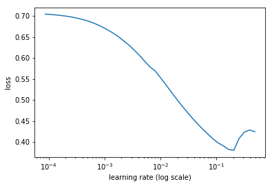
lr = 4e-2
wd = 1e-7

lrs = np.array([lr / 100, lr / 10, lr])

%time learn.fit(lr, 1, wds=wd, cycle_len=8, use_clr=(5, 8))

# -----------------------------------------------------------------------------
# Output
# -----------------------------------------------------------------------------
Epoch 100% 8/8 [03:20<00:00, 25.08s/it]

epoch      trn_loss   val_loss   mask_acc   dice
    0      0.066708   0.030094   0.986666   0.970317
    1      0.03581    0.0268     0.987201   0.973306
    2      0.026499   0.022651   0.991143   0.978611
    3      0.022736   0.024409   0.98834    0.975742
    4      0.02067    0.019966   0.991698   0.98108
    5      0.019395   0.019475   0.991706   0.98148
    6      0.018421   0.01992    0.990994   0.980779
    7      0.017531   0.018478   0.992754   0.982734
[array([0.01848]), 0.9927536495148189, 0.982733676754673]
CPU times: user 4min 2s, sys: 40.2 s, total: 4min 42s
Wall time: 3min 21s

learn.save('128urn-tmp')

learn.load('128urn-tmp')

learn.unfreeze()
learn.bn_freeze(True)

%time learn.fit(lrs / 4, 1, wds=wd, cycle_len=20, use_clr=(20, 10))

# -----------------------------------------------------------------------------
# Output
# -----------------------------------------------------------------------------
Epoch 100% 20/20 [10:16<00:00, 30.81s/it]
epoch      trn_loss   val_loss   <lambda>   dice
    0      0.016101   0.017776   0.992521   0.983324
    1      0.015925   0.018096   0.992984   0.983291
    2      0.018197   0.047329   0.987563   0.967537
    3      0.017198   0.017029   0.993005   0.984194
    4      0.015525   0.016861   0.993109   0.984405
    5      0.014776   0.016335   0.993529   0.984962
    6      0.014414   0.016253   0.993712   0.985091
    7      0.014118   0.016177   0.993633   0.98518
    8      0.013989   0.01612    0.993777   0.985277
    9      0.013846   0.016417   0.993895   0.985105
    10     0.01364    0.015978   0.993756   0.985407
    11     0.013568   0.015831   0.993784   0.985544
    12     0.013413   0.015774   0.993833   0.985651
    13     0.013295   0.015836   0.993919   0.985671
    14     0.013165   0.015741   0.99394    0.985754
    15     0.013016   0.015676   0.993802   0.985788
    16     0.012929   0.015596   0.993944   0.985933
    17     0.012834   0.015576   0.994039   0.985992
    18     0.012723   0.015523   0.993915   0.985972
    19     0.012671   0.015434   0.993951   0.986058
[array([0.01543]), 0.9939509204455784, 0.9860580409134332]
CPU times: user 11min 58s, sys: 1min 43s, total: 13min 41s
Wall time: 10min 17s

There are some more tricks we can do to make this a little bit better, but this is a good stuff. So the simple upsampling approach looked horrible and had a dice of .968. A U-Net with everything else identical except we've now got these UnetBlocks has a dice of .985! That's like we halved the error with everything else exactly the same [1:55:42]. And more the point, you can look at it.

learn.save('128urn-0')

learn.load('128urn-0')

x, y = next(iter(md.val_dl))
py = to_np(learn.model(V(x)))

This is actually looking somewhat car-like compared to our non-U-Net equivalent which is just a blob. Because trying to do this through down and up paths — it's just asking too much. Where else, when we actually provide the downward path pixels at every point, it can actually start to create something car-ish.

show_img(py[0] > 0)

show_img(y[0])

At the end of that, we'll do m.close to remove those sfs.features taking up GPU memory.

m.close()

512x512 [01:56:26]

Go to a smaller batch size, higher size.

sz=512
bs=16

tfms = tfms_from_model(resnet34, sz, crop_type=CropType.NO, tfm_y=TfmType.CLASS, aug_tfms=aug_tfms)
datasets = ImageData.get_ds(MatchedFilesDataset, (trn_x, trn_y), (val_x, val_y), tfms, path=PATH)
md = ImageData(PATH, datasets, bs, num_workers=4, classes=None) # num_workers depends on batch size

denorm = md.trn_ds.denorm

m_base = get_base()
m = to_gpu(Unet34(m_base))
models = UnetModel(m)

learn = ConvLearner(md, models)
learn.opt_fn = optim.Adam
learn.crit = nn.BCEWithLogitsLoss()
learn.metrics = [accuracy_thresh(0.5),dice]

learn.freeze_to(1)

learn.load('128urn-0')

%time learn.fit(lr, 1, wds=wd, cycle_len=8, use_clr=(20, 8))

# -----------------------------------------------------------------------------
# Output
# -----------------------------------------------------------------------------
Epoch 100% 8/8 [35:41<00:00, 267.67s/it]
epoch      trn_loss   val_loss   <lambda>   dice
    0      0.013183   0.017253   0.992196   0.983875
    1      0.014358   0.012795   0.995054   0.988391
    2      0.012857   0.012711   0.994946   0.988293
    3      0.012494   0.012167   0.995214   0.988786
    4      0.011796   0.011778   0.995447   0.989214
    5      0.011607   0.011574   0.995224   0.989329
    6      0.010983   0.010902   0.995638   0.989993
    7      0.010343   0.010676   0.995724   0.990229
[array([0.01068]), 0.9957240573943608, 0.990229018171244]
CPU times: user 43min 54s, sys: 5min 4s, total: 48min 59s
Wall time: 35min 41s

You can see the dice coefficients really going up [1:56:30]. So notice above, I'm loading in the 128x128 version of the network. We are doing this progressive resizing trick again, so that gets us .990.

learn.save('512urn-tmp-2')

learn.unfreeze()
learn.bn_freeze(True)

learn.load('512urn-tmp-2')

%time learn.fit(lrs / 4, 1, wds=wd, cycle_len=10, use_clr=(20, 10))

# -----------------------------------------------------------------------------
# Output
# -----------------------------------------------------------------------------
Epoch 100% 10/10 [57:47<00:00, 346.72s/it]
epoch      trn_loss   val_loss   mask_acc   dice
    0      0.009372   0.010585   0.995743   0.990435
    1      0.009201   0.009934   0.995893   0.990923
    2      0.022731   0.014535   0.994104   0.986531
    3      0.012456   0.012546   0.994909   0.988559
    4      0.011394   0.011722   0.995429   0.989384
    5      0.010975   0.011325   0.995433   0.989744
    6      0.010621   0.011133   0.995728   0.990007
    7      0.010379   0.011007   0.995749   0.990243
    8      0.010233   0.010774   0.995854   0.990384
    9      0.010275   0.010706   0.995858   0.990412
[array([0.01071]), 0.9958578631991432, 0.99041168513311]

CPU times: user 1h 8min 16s, sys: 6min 22s, total: 1h 14min 39s
Wall time: 57min 48s

Then unfreeze to get to .994.

📝 note-to-self: I am unable to replicate this dice score, even after trying re-train with different clr and number of cycle, so for now I proceed and need to revisit this at a later time

learn.save('512urn')

learn.load('512urn')

x, y = next(iter(md.val_dl))
py = to_np(learn.model(V(x)))

And you can see, it's now looking pretty good.

show_img(py[0] > 0)

show_img(y[0])

m.close()

1024x1024 [01:56:53]

Go down to a batch size of 4, size of 1024.

sz = 1024
bs = 4

tfms = tfms_from_model(resnet34, sz, crop_type=CropType.NO, tfm_y=TfmType.CLASS)
datasets = ImageData.get_ds(MatchedFilesDataset, (trn_x, trn_y), (val_x, val_y), tfms, path=PATH)
md = ImageData(PATH, datasets, bs, num_workers=16, classes=None)

denorm = md.trn_ds.denorm

m_base = get_base()
m = to_gpu(Unet34(m_base))
models = UnetModel(m)

learn = ConvLearner(md, models)
learn.opt_fn = optim.Adam
learn.crit = nn.BCEWithLogitsLoss()
learn.metrics = [accuracy_thresh(0.5), dice]

Load in what we just saved with the 512.

learn.load('512urn')

learn.freeze_to(1)

learn.fit(lr,1, wds=wd, cycle_len=2, use_clr=(5, 4))

# -----------------------------------------------------------------------------
# Output
# -----------------------------------------------------------------------------
Epoch 100% 2/2 [45:06<00:00, 1353.19s/it]
epoch      trn_loss   val_loss   <lambda>   dice
    0      0.013102   0.013132   0.994931   0.988265
    1      0.010119   0.011204   0.99575    0.989929
[array([0.0112]), 0.9957499636544122, 0.9899293804994912]
CPU times: user 45min 17s, sys: 6min 50s, total: 52min 8s
Wall time: 45min 6s

That gets us to .995.

📝 note-to-self: I am unable to replicate this dice score, so for now I proceed and need to revisit this at a later time.

learn.save('1024urn-tmp')

learn.load('1024urn-tmp')

learn.unfreeze()
learn.bn_freeze(True)

lrs = np.array([lr / 200, lr / 30, lr])
lrs

# -----------------------------------------------------------------------------
# Output
# -----------------------------------------------------------------------------
array([0.0002 , 0.00133, 0.04   ])

%time learn.fit(lrs / 10, 1, wds=wd, cycle_len=4, use_clr=(20, 8))

# -----------------------------------------------------------------------------
# Output
# -----------------------------------------------------------------------------
Epoch 100% 4/4 [1:52:35<00:00, 1688.95s/it]
epoch      trn_loss   val_loss   mask_acc   dice
    0      0.008753   0.010227   0.996026   0.990752
    1      0.008583   0.009887   0.996214   0.990971
    2      0.008157   0.009736   0.996149   0.991187
    3      0.008089   0.00963    0.996239   0.991263
[array([0.00963]), 0.9962390765311226, 0.9912625075008968]
CPU times: user 1h 53min, sys: 13min 28s, total: 2h 6min 28s
Wall time: 1h 52min 36s

learn.sched.plot_loss()

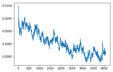
learn.sched.plot_lr()

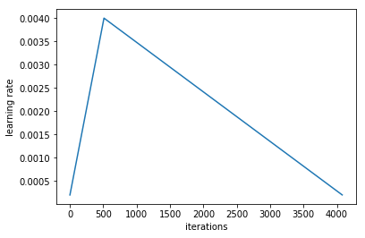
4 cycles for 4 epochs. So, 1 cycle is 1 epoch. Therefore, 1 epoch is 1000 iterations.

%time learn.fit(lrs / 10, 1, wds=wd, cycle_len=4, use_clr=(20, 8))

# -----------------------------------------------------------------------------
# Output
# -----------------------------------------------------------------------------
Epoch 100% 4/4 [1:52:23<00:00, 1685.90s/it]
epoch      trn_loss   val_loss   mask_acc   dice
    0      0.008318   0.009903   0.996072   0.991031
    1      0.008046   0.009467   0.996279   0.991389
    2      0.007842   0.009408   0.99639    0.991476
    3      0.00743    0.00936    0.996377   0.991522
[array([0.00936]), 0.9963768663860503, 0.9915224222062244]
CPU times: user 1h 52min 46s, sys: 13min 25s, total: 2h 6min 11s
Wall time: 1h 52min 24s

Unfreeze takes us to… we'll call that .996.

📝 note-to-self: I am unable to replicate this dice score, so for now I proceed and need to revisit this at a later time.

learn.sched.plot_loss()

During training, the GPU memory usage peak at 11 GB on a K80.

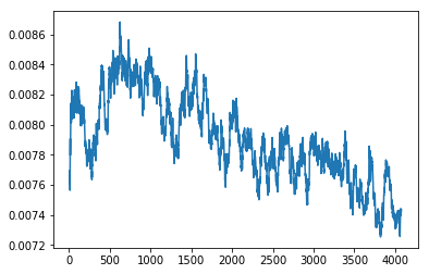
learn.save('1024urn')

learn.load('1024urn')

x, y = next(iter(md.val_dl))
py = to_np(learn.model(V(x)))

As you can see, that actually looks good [1:57:17]. In accuracy terms, 99.82%. You can see this is looking like something you could just about use to cut out. I think, at this point, there's a couple of minor tweaks we can do to get up to .997 but really the key thing then, I think, is just maybe to do a few bit of smoothing maybe or a little bit of post-processing. 🔖 You can go and have a look at the Carvana winners' blogs and see some of these tricks, but as I say, the difference between where we are at .996 and what the winners got of .997, it's not heaps. So really that just the U-Net on its own pretty much solves that problem.

show_img(py[0]>0)

show_img(y[0])

Back to Bounding Box [01:58:15]

Okay, so that's it. The last thing I wanted to mention is now to come all the way back to bounding boxes because you might remember, I said our bounding box model was still not doing very well on small objects. So hopefully you might be able to guess where I'm going to go with this which is that for the bounding box model, remember how we had at different grid cells we spat out outputs of the model. And it was those earlier ones with the small grid sizes that weren't very good. How do we fix it? U-Net it! Let's have an upward path with cross connections. So then we are just going to do a U-Net and then spit them out of that. Because now those finer grid cells have all of the information of that path, and that path, and that path, and that path for leverage. Now of course, this is deep learning so that means you can't write a paper saying we just used U-Net for bounding boxes. You have to invent a new word so this is called feature pyramid networks or FPNs. And this was used in RetinaNet paper, it was created in an earlier paper specifically about FPNs. And if memory serves correctly, they did briefly cite the U-Net paper but they kind of made it sound like it was this vaguely slightly connected thing that maybe some people could consider slightly useful. But really, FPNs are U-Nets.

I don't have an implementation of it to show you but it will be a fun thing, maybe for some of us to try and I know some of the students have been trying to get it working well on the forums. So yeah, interesting thing to try. So I think a couple of things to look at after this class as well as the other things I mentioned would be playing around with FPNs and also maybe trying Kerem's DynamicUnet. They would both be interesting things to look at.

So you guys have all been through 14 lessons of me talking at you now. So I'm sorry about that. Thanks for putting up with me. I think you're going to find it hard to find people who actually know them as much about training neural networks and practice as you do. It'll be really easy for you to overestimate how capable all these other people are and underestimate how capable you are. So the main thing I'd say is, please practice, please. Just because you don't have this constant thing getting you to come back here every Monday night now. It's very easy to kind of lose that momentum. So find ways to keep it. Organize a study group, a book reading group, or get together with some friends and work on a project, or do something more than just deciding I want to keep working on X. Unless you are kind of person who's super motivated and whenever you decide to do something, it happens. That's not me. It's like I know, for something to happen, I have to say "yes, David. In October, I will absolutely teach that course" and then it's like okay I better actually write some material. That's the only way I can get stuff to happen. So we've got a great community there on the forums. If people have ideas for ways to make it better, please tell me. If you think you can help with, if you want to create some new forum or moderated in some different way or whatever, just let me know. You can always PM me and there's a lot of projects going on through GitHub as well — lots of stuff. So I hope to see you all back here at something else and thanks so much for joining me on this journey.