Lesson 12 - DarkNet; Generative Adversarial Networks (GANs)

These are my personal notes from fast.ai course and will continue to be updated and improved if I find anything useful and relevant while I continue to review the course to study much more in-depth. Thanks for reading and happy learning!

Topics

Deep dive into the DarkNet architecture used in YOLOv3.
- Use it to better understand all the details and choices that you can make when implementing a ResNet-ish architecture.
The basic approach discussed here is what we used to win the DAWNBench competition!
Generative Adversarial Networks (GANs).
- At its heart, a different kind of loss function.
- Generator and a discriminator that battle it out, and in the process combine to create a generative model that can create highly realistic outputs.
- Wasserstein GAN variant.
  - Easier to train and more resilient to a range of hyperparameters.
- CycleGAN
  - a breakthrough idea in GANs that allows us to generate images even where we don't have direct (paired) training data.
  - the basic idea is likely to be transferable to a wide range of very valuable applications.

Lesson Resources

Website
Video
Wiki
Jupyter Notebook and code
Dataset
- CIFAR10 / direct download link (161 MB)

Assignments

Papers

Must read
- Wide Residual Networks by Sergey Zagoruyko, et. al
- YOLOv3: An Incremental Improvement by Joseph Redmon, et. al
- Unsupervised Representation Learning with Deep Convolutional Generative Adversarial Networks (DCGAN) by Alec Radford, et. al
- Wasserstein GAN (WGAN) by Martin Arjovsky, et. al
- Unpaired Image-to-Image Translation using Cycle-Consistent Adversarial Networks (CycleGAN) by Jun-Yan Zhu, et. al
- A guide to convolution arithmetic for deep learning by Vincent Dumoulin, et. al
- Deconvolution and Checkerboard Artifacts by Augustus Odena, et. al
Additional papers (optional)
- Multimodal Unsupervised Image-to-Image Translation by Xun Huang, et. al

Other Resources

Other Useful Information

PyTorch implementation of CycleGAN

My Notes

Generative Adversarial Networks (GANs)

Very hot technology but definitely deserving to be in the cutting edge deep learning part of the course because they are not quite proven to be necessarily useful for anything but they are nearly there and will definitely get there. We are going to focus on the things where they are definitely going to be useful in practice and there is a number of areas where they may turn out to be useful but we don't know yet. So I think the area that they are definitely going to be useful in practice is the kind of thing you see on the left of the slide — which is for example turning drawing into rendered pictures. This comes from a paper that just came out 2 days ago, so there's a very active research going on right now.

From the last lecture [00:01:04]: One of our diversity fellows Christine Payne has a master's in medicine from Stanford and so she had an interest in thinking what it would look like if we built a language model of medicine. One of the things we briefly touched on back in lesson 4 but didn't really talk much about last time is this idea that you can actually seed a generative language model which means you've trained a language model on some corpus and then you are going to generate some text from that language model. You can start off by feeding it a few words to say "here is the first few words to create the hidden state in the language model and generate from there please. Christine did something clever which was to seed it with a question and repeat the question three times and let it generate from there. She fed a language model lots of different medical texts and fed in questions as you see below:

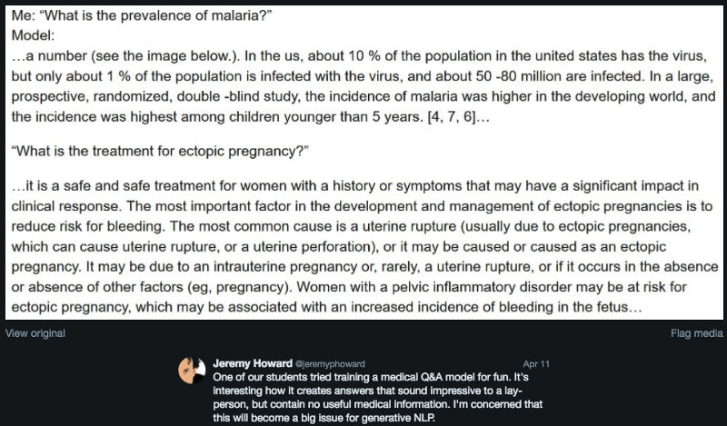
What Jeremy found interesting about this is it's pretty close to being a believable answer to the question for people without master's in medicine. But it has no bearing on reality whatsoever. He thinks it is an interesting kind of ethical and user experience quandary. Jeremy is involved in a company called doc.ai that's trying to doing a number of things but in the end provide an app for doctors and patients which can help create a conversational user interface around helping them with their medical issues. He's been continually saying to the software engineers on that team please don't try to create a generative model using LSTM or something because they are going to be really good at creating bad advice that sounds impressive — kind of like political pundits or tenured professor who can say bullcrap with great authority. So he thought it was really interesting experiment. If you've done some interesting experiments, share them in the forum, blog, Twitter. Let people know about it and get noticed by awesome people.

CIFAR10 [00:05:26]

Let's talk about CIFAR10 and the reason is that we are going to be looking at some more bare-bones PyTorch stuff today to build these generative adversarial models. There is no fastai support to speak up at all for GANs at the moment — there will be soon enough but currently there isn't so we are going to be building a lot of models from scratch. It's been a while since we've done much serious model building. We looked at CIFAR10 in the part 1 of the course and we built something which was getting about 85% accuracy and took a couple hours to train. Interestingly, there is a competition going on now to see who can actually train CIFAR10 the fastest (DAWN), and the goal is to get it to train to 94% accuracy. It would be interesting to see if we can build an architecture that can get to 94% accuracy because that is a lot better than our previous attempt. Hopefully in doing so we will learn something about creating good architectures, that will be then useful for looking at GANs today. Also it is useful because Jeremy has been looking much more deeply into the last few years' papers about different kinds of CNN architectures and realizes that a lot of the insights in those papers are not being widely leveraged and clearly not widely understood. So he wants to show you what happens if we can leverage some of that understanding.

cifar10-darknet.ipynb [00:07:17]

The notebook is called Darknet because the particular architecture we are going to look at is very close to the Darknet architecture. But you will see in the process that the Darknet architecture as in not the whole YOLO v3 end-to-end thing but just the part of it that they pre-trained on ImageNet to do classification. It's almost like the most generic simple architecture you could come up with, so it's a really great starting point for experiments. So we will call it "Darknet" but it's not quite that and you can fiddle around with it to create things that definitely aren't Darknet. It's really just the basis of nearly any modern ResNet based architecture.

CIFAR10 is a fairly small dataset [00:08:06]. The images are only 32 by 32 in size, and it's a great dataset to work with because:

You can train it relatively quickly unlike ImageNet
A relatively small amount of data
Actually quite hard to recognize the images because 32 by 32 is too small to easily see what's going on.

It is an under-appreciated dataset because it's old. Who wants to work with small old dataset when they could use their entire server room to process something much bigger. But it's is a really great dataset to focus on.

Go ahead and import our usual stuff and we are going to try and build a network from scratch to train this with [00:08:58].

%matplotlib inline
%reload_ext autoreload
%autoreload 2

from fastai.conv_learner import *

PATH = Path('data/cifar10/')
os.makedirs(PATH, exist_ok=True)
torch.backends.cudnn.benchmark = True # cut down training duration from ~3 hr to ~1hr

A really good exercise for anybody who is not 100% confident with their broadcasting and PyTorch basic skill is figure out how Jeremy came up with these stats numbers. These numbers are the averages and standard deviations for each channel in CIFAR10. Try and make sure you can recreate those numbers and see if you can do it with no more than a couple of lines of code (no loops!).

Because these are fairly small, we can use a larger batch size than usual and the size of these images is 32 [00:09:46].

classes = ('plane', 'car', 'bird', 'cat', 'deer', 'dog', 'frog', 'horse', 'ship', 'truck')

# these numbers are the averages and standard deviations for each channel in CIFAR10
stats = (np.array([ 0.4914 ,  0.48216,  0.44653]), np.array([ 0.24703,  0.24349,  0.26159]))

num_workers = num_cpus() // 2 # num cpus returns 4
bs = 256
sz = 32

Transformations [00:09:57], normally we have this standard set of side_on transformations we use for photos of normal objects. We are not going to use that here because these images are so small that trying to rotate a 32 by 32 image a bit is going to introduce a lot of blocky distortions. So the standard transformations that people tend to use is a random horizontal flip and then we add 4 pixels (size divided by 8) of padding on each side. One thing which works really well is by default fastai does not add black padding which many other libraries do. Fastai takes the last 4 pixels of the existing photo and flip it and reflect it, and we find that we get much better results by using reflection padding by default. Now that we have 40 by 40 image, this set of transforms in training will randomly pick a 32 by 32 crops, so we get a little bit of variation but not heaps. Wo we can use the normal from_paths to grab our data.

tfms = tfms_from_stats(stats, sz, aug_tfms=[RandomFlip()], pad=sz // 8)
data = ImageClassifierData.from_paths(PATH, val_name='test', tfms=tfms, bs=bs)

Now we need an architecture and we are going to create one which fits in one screen [00:11:07]. This is from scratch. We are using predefined Conv2d, BatchNorm2d, LeakyReLU modules but we are not using any blocks or anything. The entire thing is in one screen so if you are ever wondering can I understand a modern good quality architecture, absolutely! Let's study this one.

def conv_layer(ni, nf, ks=3, stride=1):
    return nn.Sequential(
        nn.Conv2d(in_channels=ni, out_channels=nf, kernel_size=ks, bias=False, stride=stride, padding=ks // 2),
        nn.BatchNorm2d(num_features=nf, momentum=0.01),
        nn.LeakyReLU(negative_slope=0.1, inplace=True)
    )

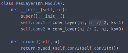
class `ResLayer`(nn.Module):
    def __init__(self, ni):
        super().__init__()
        self.conv1 = conv_layer(ni, ni // 2, ks=1)
        self.conv2 = conv_layer(ni // 2, ni, k2=3)

    def forward(self, x):
        return x.add_(self.conv2(self.conv1(x)))

class Darknet(nn.Module):
    def make_group_layer(self, ch_in, num_blocks, stride=1):
        return [conv_layer(ch_in, ch_in * 2, stride=stride)
               ] + [(ResLayer(ch_in * 2)) for i in range(num_blocks)]

    def __init__(self, num_blocks, num_classes, nf=32):
        super().__init__()
        layers = [conv_layer(3, nf, ks=3, stride=1)]
        for i, nb in enumerate(num_blocks):
            layers += self.make_group_layer(nf, nb, stride=2 - (i == 1))
            nf *= 2
        layers += [nn.AdaptiveAvgPool2d(1), Flatten(), nn.Linear(nf, num_classes)]
        self.layers = nn.Sequential(*layers)

    def forward(self, x):
        return self.layers(x)

The basic starting point with an architecture is to say it's a stacked bunch of layers and generally speaking there is going to be some kind of hierarchy of layers [00:11:51]. At the very bottom level, there is things like a convolutional layer and a batch norm layer, but any time you have a convolution, you are probably going to have some standard sequence. Normally it's going to be:

conv
batch norm
a nonlinear activation (e.g. ReLU)

We will start by determining what our basic unit is going to be and define it in a function (conv_layer) so we don't have to worry about trying to keep everything consistent and it will make everything a lot simpler.

Leaky ReLU [00:12:43]:

The gradient of Leaky ReLU (where x < 0) varies but something about 0.1 or 0.01 is common. The idea behind it is that when you are in the negative zone, you don't end up with a zero gradient which makes it very hard to update it. In practice, people have found Leaky ReLU more useful on smaller datasets and less useful in big datasets. But it is interesting that for the YOLO v3 paper, they used Leaky ReLU and got great performance from it. It rarely makes things worse and it often makes things better. So it's probably not bad if you need to create your own architecture to make that your default go-to is to use Leaky ReLU.

You'll notice that we don't define PyTorch module in conv_layer, we just do nn.Sequential [00:14:07]. This is something if you read other people's PyTorch code, it's really underutilized. People tend to write everything as a PyTorch module with __init__ and forward, but if the thing you want is just a sequence of things one after the other, it's much more concise and easy to understand to make it a Sequential.

Residual block [00:14:40]:

As mentioned before that there is generally a number of hierarchies of units in most modern networks, and we know now that the next level in this unit hierarchy for ResNet is the ResBlock or residual block (see ResLayer). Back when we last did CIFAR10, we oversimplified this (cheated a little bit). We had x coming in and we put that through a conv, then we added it back up to x to go out. In the real ResBlock, there are two of them. When we say "conv" we are using it as a shortcut for our conv_layer (conv, batch norm, ReLU).

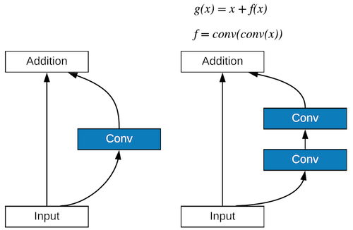
One interesting insight here is the number of channels in these convolutions [00:16:47]. We have some ni coming in (some number of input channels/filters). The way the darknet folks set things up is they make every one of these Res layers spit out the same number of channels that came in, and Jeremy liked that and that's why he used it in ResLayer because it makes life simpler. The first conv halves the number of channels, and then second conv doubles it again. So you have this funneling effect where 64 channels coming in, squished down with a first conv down to 32 channels, and then taken back up again to 64 channels coming out.

❓ Why is inplace=True in the LeakyReLU [00:17:54]?

Thanks for asking! A lot of people forget this or don't know about it, but this is a really important memory technique. If you think about it, this conv_layer, it's the lowest level thing, so pretty much everything in our ResNet once it's all put together is going to be many conv_layer's. If you do not have inplace = True, it's going to create a whole separate piece of memory for the output of the ReLU so it's going to allocate a whole bunch of memory that is totally unnecessary. Another example is that the original forward in ResLayer looked like:

def forward(self, x):
    return x + self.conv2(self.conv1(x))

Hopefully some of you might remember that in PyTorch pretty much every every function has an underscore suffix version which tells it to do it in-place. + is equivalent to add and in-place version of add is add_ so this will reduce memory usage:

def forward(self, x):
    return x.add_(self.conv2(self.conv1(x)))

These are really handy little tricks. Jeremy forgot the inplace = True at first but he was having to decrease the batch size to much lower amounts and it was driving him crazy — then he realized that that was missing. You can also do that with dropout if you have dropout. Here are what to look out for:

Dropout
All the activation functions
Any arithmetic operation

❓ In ResNet, why is bias usually set to False in conv_layer [00:19:53]?

Immediately after the Conv, there is a BatchNorm. Remember, BatchNorm has 2 learnable parameters for each activation — the thing you multiply by and the thing you add. If we had bias in Conv and then add another thing in BatchNorm, we would be adding two things which is totally pointless — that's two weights where one would do. So if you have a BatchNorm after a Conv, you can either tell BatchNorm not to include the add bit or easier is to tell Conv not to include the bias. There is no particular harm, but again, it's going to take more memory because that is more gradients that it has to keep track of, so best to avoid.

Also another little trick is, most people's conv_layer's have padding as a parameter [00:21:11]. But generally speaking, you should be able to calculate the padding easily enough. If you have a kernel size of 3, then obviously that is going to overlap by one unit on each side, so we want padding of 1. Or else, if it's kernel size of 1, then we don't need any padding. So in general, padding of kernel size "integer divided" by 2 is what you need. There're some tweaks sometimes but in this case, this works perfectly well. Again, trying to simplify my code by having the computer calculate stuff for me rather than me having to do it myself.

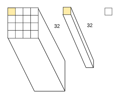
Another thing with the two conv_layer's [00:22:14]: We had this idea of bottleneck (reducing the channels and then increase them again), there is also what kernel size to use. The first one has 1 by 1 Conv. What actually happen in 1 by 1 conv? If we have 4 by 4 grid with 32 filters/channels and we will do 1 by 1 conv, the kernel for the conv looks like the one in the middle. When we talk about the kernel size, we never mention the last piece — but let's say it's 1 by 1 by 32 because that's the part of the filters in and filters out. The kernel gets placed on the first cell in yellow and we get a dot product these 32 deep bits which gives us our first output. We then move it to the second cell and get the second output. So there will be bunch of dot products for each point in the grid. It is allowing us to change the dimensionality in whatever way we want in the channel dimension. We are creating ni//2 filters and we will have ni//2 dot products which are basically different weighted averages of the input channels. With very little computation, it lets us add this additional step of calculations and nonlinearities. It is a cool trick to take advantage of these 1 by 1 convs, creating this bottleneck, and then pulling it out again with 3 by 3 convs — which will take advantage of the 2D nature of the input properly. Or else, 1 by 1 conv doesn't take advantage of that at all.

These two lines of code, there is not much in it, but it's a really great test of your understanding and intuition about what is going on [00:25:17] — why does it work? why do the tensor ranks line up? why do the dimensions all line up nicely? why is it a good idea? what is it really doing? It's a really good thing to fiddle around with. Maybe create some small ones in Jupyter Notebook, run them yourself, see what inputs and outputs come in and out. Really get a feel for that. Once you've done so, you can then play around with different things.

Wide Residual Networks

One of the really unappreciated papers is this one [00:26:09] — Wide Residual Networks. It's really quite simple paper but what they do is they fiddle around with these two lines of code:

What if we did ni*2 instead of ni//2?
What if we added conv3?

They come up with this kind of simple notation for defining what the two lines of code can look like and they show lots of experiments. What they show is that this approach of a bottlenecking of decreasing the number of channels which is almost universal in ResNet is probably not a good idea. In fact, from the experiments, definitely not a good idea. Because what happens is it lets you create really deep networks. The guys who created ResNet got particularly famous for creating 1001 layer network. But the thing about 1001 layers is you can't calculate layer 2 until you are finished layer 1. You can't calculate layer 3 until you finish calculating layer 2. So it's sequential. GPUs don't like sequential. So what they showed is that if you have less layers but with more calculations per layer — so one easy way to do that would be to remove //2, no other changes:

self.conv1 = conv_layer(ni, ni, ks=1)
self.conv2 = conv_layer(ni, ni, ks=3)

🔖 Try this at home. Try running CIFAR and see what happens. Even multiply by 2 or fiddle around.

That lets your GPU do more work and it's very interesting because the vast majority of papers that talk about performance of different architectures never actually time how long it takes to run a batch through it. They say "this one takes X number of floating-point operations per batch" but they never actually bother to run it like a proper experimentalists and find out whether it's faster or slower. A lot of the architectures that are really famous now turn out to be slow as molasses and take crap loads of memory and just totally useless because the researchers never actually bothered to see whether they are fast and to actually see whether they fit in RAM with normal batch sizes.

So Wide ResNet paper is unusual in that it actually times how long it takes as does the YOLO v3 paper which made the same insight. They might have missed the Wide ResNet paper because the YOLO v3 paper came to a lot of the same conclusions but Jeremy is not sure they cited the Wide ResNet paper so they might not be aware that all that work has been done. It's great to see people are actually timing things and noticing what actually makes sense.

❓ What is your opinion on SELU (scaled exponential linear units)? [00:29:44]

SELU is largely for fully connected layers which allows you to get rid of batch norm and the basic idea is that if you use this different activation function, it's self normalizing. Self normalizing means it will always remain at a unit standard deviation and zero mean and therefore you don't need batch norm. It hasn't really gone anywhere and the reason is because it's incredibly finicky — you have to use a very specific initialization otherwise it doesn't start with exactly the right standard deviation and mean. Very hard to use it with things like embeddings, if you do then you have to use a particular kind of embedding initialization which doesn't make sense for embeddings. And you do all this work, very hard to get it right, and if you do finally get it right, what's the point? Well, you've managed to get rid of some batch norm layers which weren't really hurting you anyway. It's interesting because the SELU paper — the main reason people noticed it was because it was created by the inventor of LSTM and also it had a huge mathematical appendix. So people thought "lots of maths from a famous guy — it must be great!" but in practice, Jeremy doesn't see anybody using it to get any state-of-the-art results or win any competitions.

Darknet.make_group_layer contains a bunch of ResLayer [00:31:28]. group_layer is going to have some number of channels/filters coming in. We will double the number of channels coming in by just using the standard conv_layer. Optionally, we will halve the grid size by using a stride of 2. Then we are going to do a whole bunch of ResLayers — we can pick how many (2, 3, 8, etc) because remember ResLayers do not change the grid size and they don't change the number of channels, so you can add as many as you like without causing any problems. This is going to use more computation and more RAM but there is no reason other than that you can't add as many as you like. group_layer, therefore, is going to end up doubling the number of channels because the initial convolution doubles the number of channels and depending on what we pass in as stride, it may also halve the grid size if we put stride=2. And then we can do a whole bunch of Res block computations as many as we like.

To define our Darknet, we are going to pass in something that looks like this [00:33:13]:

m = Darknet([1, 2, 4, 6, 3], num_classes=10, nf=32)
m = nn.DataParallel(m, [1, 2, 3]) # disabled this line if you have single GPU

What this says is create five group layers: the first one will contain 1 extra ResLayer, the second will contain 2, then 4, 6, 3 and we want to start with 32 filters. The first one of ResLayers will contain 32 filters, and there'll just be one extra ResLayer. The second one, it's going to double the number of filters because that's what we do each time we have a new group layer. So the second one will have 64, and then 128, 256, 512 and that'll be it. Nearly all of the network is going to be those bunches of layers and remember, every one of those group layers also has one convolution at the start. So then all we have is before that all happens, we are going to have one convolutional layer at the very start, and at the very end we are going to do our standard adaptive average pooling, flatten, and a linear layer to create the number of classes out at the end. To summarize [00:34:44], one convolution at one end, adaptive pooling and one linear layer at the other end, and in the middle, these group layers each one consisting of a convolutional layer followed by n number of ResLayers.

Adaptive average pooling [00:35:02]: Jeremy's mentioned this a few times, but he's yet to see any code out there, any example, anything anywhere, that uses adaptive average pooling. Every one he's seen writes it like nn.AvgPool2d(n) where n is a particular number — this means that it's now tied to a particular image size which definitely isn't what you want. So most people are still under the impression that a specific architecture is tied to a specific size (size here means the input size. i.e image size 32 by 32). That's a huge problem when people think that because it really limits their ability to use smaller sizes to kick-start their modeling or to use smaller size for doing experiments.

Sequential [00:35:53]: A nice way to create architectures is to start out by creating a list, in this case this is a list with just one conv_layer in, and make_group_layer returns another list. Then we can append that list to the previous list with += and do the same for another list containing AdaptiveAvgPool2d. Finally we will call nn.Sequential of all those layers. Now the forward is just self.layers(x).

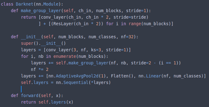
This is a nice picture of how to make your architectures as simple as possible. There are a lot you can fiddle around with. You can parameterize the divider of ni to make it a number that you pass in to pass in different numbers- maybe do times 2 instead. You can also pass in things that change the kernel size, or change the number of convolutional layers. Jeremy has a version of this which he is going to run for you which implements all of the different parameters that were in the Wide ResNet paper, so he could fiddle around to see what worked well.

lr = 1.3

learn = ConvLearner.from_model_data(m, data)
learn.crit = nn.CrossEntropyLoss()
learn.metrics = [accuracy]
wd = 1e-4

Once we've got that, we can use ConvLearner.from_model_data to take our PyTorch module and a model data object, and turn them into a learner [00:37:08]. Give it a criterion, add a metrics if we like, and then we can fit and away we go.

%time learn.fit(lr, 1, wds=wd, cycle_len=30, use_clr_beta=(20, 20, 0.95, 0.85))

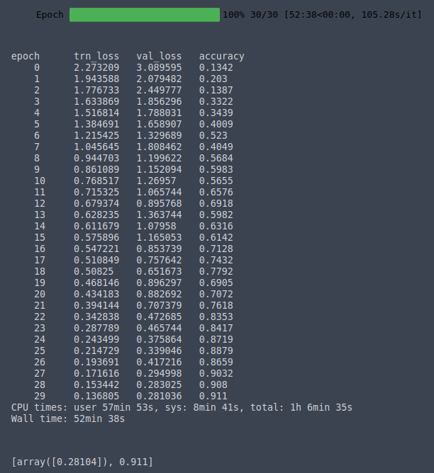
📝 On my server with a single Tesla K80, I am able to train to 91% accuracy in 52 minutes 38 seconds.

❓ Could you please explain adaptive average pooling? How does setting to 1 work [00:37:25]?

Sure. Normally when we are doing average pooling, let's say we have 4x4 and we did avgpool((2, 2)) [00:40:35]. That creates 2x2 area (blue in the below) and takes the average of those four. If we pass in stride=1, the next one is 2x2 shown in green and take the average. So this is what a normal 2x2 average pooling would be. If we didn't have any padding, that would spit out 3x3. If we wanted 4x4, we can add padding.

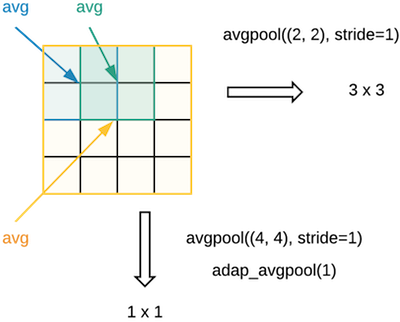
What if we wanted 1x1? Then we could say avgpool((4,4), stride=1) that would do 4x4 in yellow and average the whole lot which results in 1x1. But that's just one way to do it. Rather than saying the size of the pooling filter, why don't we instead say "I don't care what the size of the input grid is. I always want one by one". That's where you say adap_avgpool(1). In this case, you don't say what's the size of the pooling filter, you instead say what the size of the output we want. We want something that's one by one. If you put a single integer n, it assumes you mean n by n. In this case, adaptive average pooling 1 with a 4x4 grid coming in is the same as average pooling (4, 4). If it was 7x7 grid coming in, it would be the same as average pooling (7, 7). It is the same operation, it's just expressing it in a way that regardless of the input, we want something of that sized output.

DAWNBench [00:37:43]

Let's see how we go with our simple network against these state-of-the-art results. Jeremy has the command ready to go. We've taken all that stuff and put it into a simple Python script, and he modified some of the parameters he mentioned to create something he called wrn_22 network which doesn't officially exist but it has a bunch of changes to the parameters we talked about based on Jeremy's experiments. It has bunch of cool stuff like:

Leslie Smith's one cycle
Half-precision floating-point implementation

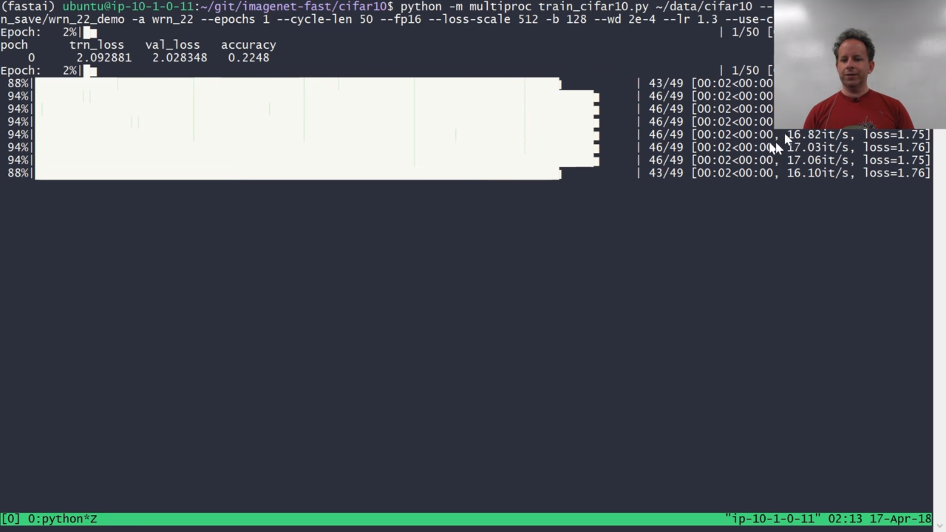
This is going to run on AWS p3 which has 8 GPUs and Volta architecture GPUs which have special support for half-precision floating-point. Fastai is the first library to actually integrate the Volta optimized half-precision floating-point into the library, so you can just do learn.half() and get that support automatically. And it's also the first to integrate one cycle.

What this actually does is it's using PyTorch's multi-GPU support [00:39:35]. Since there are eight GPUs, it is actually going to fire off eight separate Python processes and each one is going to train on a little bit and then at the end it's going to pass the gradient updates back to the master process that is going to integrate them all together. So you will see lots of progress bars pop up together.

You can see it's training three or four seconds when you do it this way. Where else, when Jeremy was training earlier, he was getting 30 seconds per epoch. So doing it this way, we can train things ~10 times faster which is pretty cool.

Checking on the status [00:43:19]:

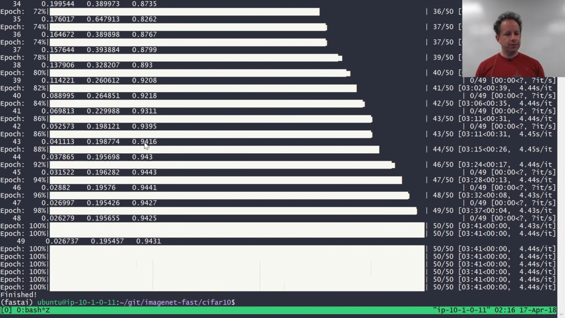
It's done! We got to 94% and it took 3 minutes and 11 seconds. Previous state-of-the-art was 1 hour 7 minutes. Was it worth fiddling around with those parameters and learning a little bit about how these architectures actually work and not just using what came out of the box? Well, holy crap. We just used a publicly available instance (we used a spot instance so it costs us $8 per hour — for 3 minutes, 40 cents) to train this from scratch 20 times faster than anybody has ever done it before. So that is one of the craziest state-of-the-art result. We've seen many but this one just blew it out of the water. This is partly thanks to fiddling around with those parameters of the architecture, mainly frankly about using Leslie Smith's one cycle. Reminder of what it is doing [00:44:35], for learning rate, it creates upward path that is equally long as the downward path so it's true triangular cyclical learning rate (CLR). As per usual, you can pick the ratio of x and y (i.e. starting LR / peak LR).

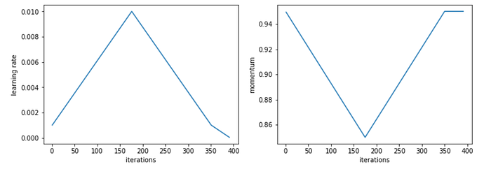
In this case, we picked 50 for the ratio. So we started out with much smaller learning rate. Then it has this cool idea where you get to say what percentage of your epochs is spent going from the bottom of the triangle all the way down pretty much to zero — that is the second number. So 15% of the batches are spent going from the bottom of our triangle even further.

That is not the only thing one cycle does, we also have momentum. Momentum goes from .95 to .85. In other words, when learning rate is really low, we use a lot of momentum and when the learning rate is really high, we use very little momentum which makes a lot of sense but until Leslie Smith showed this in the paper, Jeremy has never seen anybody do it before. It's a really cool trick. You can now use that by using use-clr-beta parameter in fastai (forum post by Sylvain) and you should be able to replicate the state-of-the-art result. You can use it on your own computer or your Paperspace, the only thing you won't get is the multi-GPU piece, but that makes it a bit easier to train anyway.

❓ make_group_layer contains stride equals 2, so this means stride is one for layer one and two for everything else. What is the logic behind it?

Usually the strides I have seen are odd [00:46:52]. Strides are either one or two. I think you are thinking of kernel sizes. So stride=2 means that I jump two across which means that you halve your grid size. So I think you might have got confused between stride and kernel size there. If you have a stride of one, the grid size does not change. If you have a stride of two, then it does. In this case, because this is CIFAR10, 32 by 32 is small and we don't get to halve the grid size very often because pretty quickly we are going to run out of cells. So that is why the first layer has a stride of one so we don't decrease the grid size straight away. It is kind of a nice way of doing it because that's why we have a low number at first Darknet([1, 2, 4, 6, 3], …) . We can start out with not too much computation on the big grid, and then we can gradually doing more and more computation as the grids get smaller and smaller because the smaller grid the computation will take less time.

Generative Adversarial Networks (GAN) [00:48:49]

We are going to talk about generative adversarial networks also known as GANs and specifically we are going to focus on Wasserstein GAN paper which included Soumith Chintala who went on to create PyTorch. Wasserstein GAN (WGAN) was heavily influenced by the deep convolutional generative adversarial network paper which also Soumith was involved with. It is a really interesting paper to read. A lot of it looks like this:

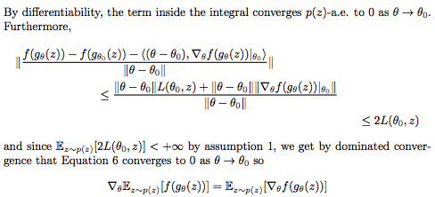
The good news is you can skip those bits because there is also a bit that looks like this:

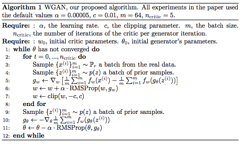
A lot of papers have a theoretical section which seems to be there entirely to get past the reviewer's need for theory. That's not true with WGAN paper. The theory bit is actually interesting — you don't need to know it to use it, but if you want to learn about some cool ideas and see the thinking behind why this particular algorithm, it's absolutely fascinating. Before this paper came out, Jeremy knew nobody who studied the math it's based on, so everybody had to learn the math. The paper does a pretty good job of laying out all the pieces (you have to do a bunch of reading yourself). So if you are interested in digging into the deeper math behind some paper to see what it's like to study it, I would pick this one because at the end of that theory section, you'll come away saying "I can see now why they made this algorithm the way it is."

The basic idea of GAN is it's a generative model[00:51:23]. It is something that is going to create sentences, create images, or generate something. It is going to try and create thing which is very hard to tell the difference between generated stuff and real stuff. So generative model could be used to face-swap a video — a very controversial thing of deep fakes and fake pornography happening at the moment. It could be used to fake somebody's voice. It could be used to fake the answer to a medical question — but in that case, it's not really a fake, it could be a generative answer to a medical question that is actually a good answer so you are generating language. You could generate a caption to an image, for example. So generative models have lots of interesting applications. But generally speaking, they need to be good enough that for example if you are using it to automatically create a new scene for Carrie Fisher in the next Star Wars movie and she is not around to play that part anymore, you want to try and generate an image of her that looks the same then it has to fool the Star Wars audience into thinking "okay, that doesn't look like some weird Carrie Fisher — that looks like the real Carrie Fisher. Or if you are trying to generate an answer to a medical question, you want to generate English that reads nicely and clearly, and sounds authoritative and meaningful. The idea of generative adversarial network is we are going to create not just a generative model to create the generated image, but a second model that's going to try to pick which ones are real and which ones are generated (we will call them "fake"). So we have a generator that is going to create our fake content and a discriminator that's going to try to get good at recognizing which ones are real and which ones are fake. So there are going to be two models and they are going to be adversarial, meaning the generator is going to try to keep getting better at fooling the discriminator into thinking that fake is real, and the discriminator is going to try to keep getting better at discriminating between the real and the fake. So they are going to go head to head. It is basically as easy as Jeremy just described [00:54:14]:

We are going to build two models in PyTorch
We are going to create a training loop that first of all says the loss function for the discriminator is "can you tell the difference between real and fake, then update the weights of that".
We are going to create a loss function for the generator which is "can you generate something which fools the discriminator and update the weights from that loss".
And we are going to loop through that a few times and see what happens.

Looking at the code [00:54:52]

wgan.ipynb

There is a lot of different things you can do with GANS. We are going to do something that is kind of boring but easy to understand and it's kind of cool that it's even possible which is we are going to generate some pictures from nothing. We are just going to get it to draw some pictures. Specifically, we are going to get it to draw pictures of bedrooms. Hopefully you get a chance to play around with this during the week with your own datasets. If you pick a dataset that's very varied like ImageNet and then get a GAN to try and create ImageNet pictures, it tends not to do so well because it's not clear enough what you want a picture of. So it's better to give it, for example, there is a dataset called CelebA which is pictures of celebrities' faces that works great with GANs. You create really clear celebrity faces that don't actually exist. The bedroom dataset is also a good one — pictures of the same kind of thing.

There is something called LSUN scene classification dataset [00:55:55].

from fastai.conv_learner import *
from fastai.dataset import *
import gzip

Download the LSUN scene classification dataset bedroom category, unzip it, and convert it to JPG files (the scripts folder is here in the dl2 folder):

%mkdir data/lsun
%cd data/lsun

!aria2c --file-allocation=none -c -x 5 -s 5 'http://lsun.cs.princeton.edu/htbin/download.cgi?tag=latest&category=bedroom&set=train'

!unzip bedroom_train_lmdb.zip

%cd ~/fastai/courses/dl2/

!pip install lmdb

!python lsun_scripts/lsun-data.py data/lsun/bedroom_train_lmdb --out_dir data/lsun/bedroom

This isn't tested on Windows - if it doesn't work, you could use a Linux box to convert the files, then copy them over. Alternatively, you can download this 20% sample from Kaggle datasets.

PATH = Path('data/lsun')
IMG_PATH = PATH / 'bedroom'
CSV_PATH = PATH / 'files.csv'
TMP_PATH = PATH / 'tmp'
TMP_PATH.mkdir(exist_ok=True)

In this case, it is much easier to go the CSV route when it comes to handling our data. So we generate a CSV with the list of files that we want, and a fake label "0" because we don't really have labels for these at all. One CSV file contains everything in that bedroom dataset, and another one contains random 10%. It is nice to do that because then we can most of the time use the sample when we are experimenting because there is well over a million files even just reading in the list takes a while.

files = PATH.glob('bedroom/**/*.jpg')

with CSV_PATH.open('w') as fo:
    for f in files:
        fo.write(f'{f.relative_to(IMG_PATH)}, 0\n')

# Optional - sampling a subset of files
CSV_PATH = PATH/'files_sample.csv'

files = PATH.glob('bedroom/**/*.jpg')

with CSV_PATH.open('w') as fo:
    for f in files:
        if random.random() < 0.1:
            fo.write(f'{f.relative_to(IMG_PATH)},0\n')

This will look pretty familiar [00:57:10]. This is before Jeremy realized that sequential models are much better. So if you compare this to the previous conv block with a sequential model, there is a lot more lines of code here — but it does the same thing of conv, ReLU, batch norm.

class ConvBlock(nn.Module):
    def __init__(self, ni, no, ks, stride, bn=True, pad=None):
        super().__init__()
        if pad is None:
            pad = ks // 2 // stride
        self.conv = nn.Conv2d(ni, no, ks, stride, padding=pad, bias=False)
        self.bn = nn.BatchNorm2d(no) if bn else None
        self.relu = nn.LeakyReLU(0.2, inplace=True)

    def forward(self, x):
        x = self.relu(self.conv(x))
        return self.bn(x) if self.bn else x

Discriminator

The first thing we are going to do is to build a discriminator [00:57:47]. A discriminator is going to receive an image as an input, and it's going to spit out a number. The number is meant to be lower if it thinks this image is real. Of course "what does it do for a lower number" thing does not appear in the architecture, that will be in the loss function. So all we have to do is to create something that takes an image and spits out a number. A lot of this code is borrowed from the original authors of this paper, so some of the naming scheme is different to what we are used to. But it looks similar to what we had before. We start out with a convolution (conv, ReLU, batch norm). Then we have a bunch of extra conv layers — this is not going to use a residual so it looks very similar to before a bunch of extra layers but these are going to be conv layers rather than res layers. At the end, we need to append enough stride 2 conv layers that we decrease the grid size down to no bigger than 4x4. So it's going to keep using stride 2, divide the size by 2, and repeat till our grid size is no bigger than 4. This is quite a nice way of creating as many layers as you need in a network to handle arbitrary sized images and turn them into a fixed known grid size.

❓ Does GAN need a lot more data than say dogs vs. cats or NLP? Or is it comparable [00:59:48]?

Honestly, I am kind of embarrassed to say I am not an expert practitioner in GANs. The stuff I teach in part one is things I am happy to say I know the best way to do these things and so I can show you state-of-the-art results like we just did with CIFAR10 with the help of some of the students. I am not there at all with GANs so I am not quite sure how much you need. In general, it seems it needs quite a lot but remember the only reason we didn't need too much in dogs and cats is because we had a pre-trained model and could we leverage pre-trained GAN models and fine tune them? Probably. I don't think anybody has done it as far as I know. That could be really interesting thing for people to think about and experiment with. Maybe people have done it and there is some literature there we haven't come across. I'm somewhat familiar with the main pieces of literature in GANs but I don't know all of it, so maybe I've missed something about transfer learning in GANs. But that would be the trick to not needing too much data.

❓ So the huge speed-up a combination of one cycle learning rate and momentum annealing plus the eight GPU parallel training in the half precision? Is that only possible to do the half precision calculation with consumer GPU? Another question, why is the calculation 8 times faster from single to half precision, while from double the single is only 2 times faster [1:01:09]?

Okay, so the CIFAR10 result, it's not 8 times faster from single to half. It's about 2 or 3 times as fast from single to half. NVIDIA claims about the flops performance of the tensor cores, academically correct, but in practice meaningless because it really depends on what calls you need for what piece — so about 2 or 3x improvement for half. So the half precision helps a bit, the extra GPUs helps a bit, the one cycle helps an enormous amount, then another key piece was the playing around with the parameters that I told you about. So reading the wide ResNet paper carefully, identifying the kinds of things that they found there, and then writing a version of the architecture you just saw that made it really easy for us to fiddle around with parameters, staying up all night trying every possible combination of different kernel sizes, numbers of kernels, number of layer groups, size of layer groups. And remember, we did a bottleneck but actually we intended to focus instead on widening so we increase the size and then decrease it because it takes better advantage of the GPU. So all those things combined together, I'd say the one cycle was perhaps the most critical but every one of those resulted in a big speed-up. That's why we were able to get this 30x improvement over the state-of-the-art CIFAR10. We have some ideas for other things — after this DAWNBench finishes, maybe we'll try and go even further to see if we can beat one minute one day. That'll be fun.

class DCGAN_D(nn.Module):
    def __init__(self, isize, nc, ndf, n_extra_layers=0):
        super().__init__()
        assert isize % 16 == 0, "isize has to be a multiple of 16"

        self.initial = ConvBlock(nc, ndf, 4, 2, bn=False)
        csize, cndf = isize / 2, ndf
        self.extra = nn.Sequential(*[ConvBlock(cndf, cndf, 3, 1)
                                    for t in range(n_extra_layers)])

        pyr_layers = [] # pyramid layers
        while csize > 4:
            pyr_layers.append(ConvBlock(cndf, cndf * 2, 4, 2))
            cndf *= 2
            csize /= 2
        self.pyramid = nn.Sequential(*pyr_layers)

        self.final = nn.Conv2d(cndf, 1, 4, padding=0, bias=False)

    def forward(self, input):
        x = self.initial(input)
        x = self.extra(x)
        x = self.pyramid(x)
        return self.final(x).mean(0).view(1)

So here is our discriminator [1:03:37].The important thing to remember about an architecture is it doesn't do anything rather than have some input tensor size and rank, and some output tensor size and rank. As you see the last conv has one channel. This is different from what we are used to because normally our last thing is a linear block. But our last layer here is a conv block. It only has one channel but it has a grid size of something around 4x4 (no more than 4x4). So we are going to spit out (let's say it's 4x4), 4 by 4 by 1 tensor. What we then do is we then take the mean of that. So it goes from 4x4x1 to a scalar. This is kind of like the ultimate adaptive average pooling because we have something with just one channel and we take the mean. So this is a bit different — normally we first do average pooling and then we put it through a fully connected layer to get our one thing out. But this is getting one channel out and then taking the mean of that. Jeremy suspects that it would work better if we did the normal way, but he hasn't tried it yet and he doesn't really have a good enough intuition to know whether he is missing something — but 🔖 it will be an interesting experiment to try if somebody wants to stick an adaptive average pooling layer and a fully connected layer afterwards with a single output.

So that's a discriminator. Let's assume we already have a generator — somebody says "okay, here is a generator which generates bedrooms. I want you to build a model that can figure out which ones are real and which ones aren't". We are going to take the dataset and label bunch of images which are fake bedrooms from the generator, and a bunch of images of real bedrooms from LSUN dataset to stick a 1 or a 0 on each one. Then we'll try to get the discriminator to tell the difference. So that is going to be simple enough. But we haven't been given a generator. We need to build one. We haven't talked about the loss function yet — we are going to assume that there's some loss function that does this thing.

Generator [1:06:15]

A generator is also an architecture which doesn't do anything by itself until we have a loss function and data. But what are the ranks and sizes of the tensors? The input to the generator is going to be a vector of random numbers. In the paper, they call that the "prior." How big? We don't know. The idea is that a different bunch of random numbers will generate a different bedroom. So our generator has to take as input a vector, stick it through sequential models, and turn it into a rank 4 tensor (rank 3 without the batch dimension) — height by width by 3. So in the final step, nc (number of channel) is going to have to end up being 3 because it's going to create a 3 channel image of some size.

class DeconvBlock(nn.Module):
    def __init__(self, ni, no, ks, stride, pad, bn=True):
        super().__init__()
        self.conv = nn.ConvTranspose2d(ni, no, ks, stride, padding=pad, bias=False)
        self.bn = nn.BatchNorm2d(no)
        self.relu = nn.ReLU(inplace=True)

    def forward(self, x):
        x = self.relu(self.conv(x))
        return self.bn(x) if self.bn else x

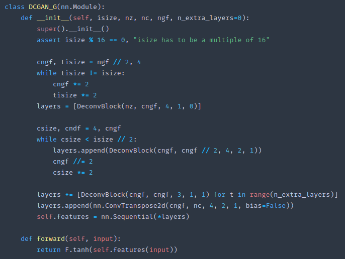
class DCGAN_G(nn.Module):
    def __init__(self, isize, nz, nc, ngf, n_extra_layers=0):
        super().__init__()
        assert isize % 16 == 0, "isize has to be a multiple of 16"

        cngf, tisize = ngf // 2, 4
        while tisize != isize:
            cngf *= 2
            tisize *= 2
        layers = [DeconvBlock(nz, cngf, 4, 1, 0)]

        csize, cndf = 4, cngf
        while csize < isize // 2:
            layers.append(DeconvBlock(cngf, cngf // 2, 4, 2, 1))
            cngf //= 2
            csize *= 2

        layers += [DeconvBlock(cngf, cngf, 3, 1, 1) for t in range(n_extra_layers)]
        layers.append(nn.ConvTranspose2d(cngf, nc, 4, 2, 1, bias=False))
        self.features = nn.Sequential(*layers)

    def forward(self, input):
        return F.tanh(self.features(input))

❓ In ConvBlock, is there a reason why batch norm comes after ReLU (i.e. self.bn(self.relu(…))) [1:07:50]?

I would normally expect to go ReLU then batch norm [1:08:23] that this is actually the order that makes sense to Jeremy. The order we had in the DarkNet was what they used in the DarkNet paper, so everybody seems to have a different order of these things. In fact, most people for CIFAR10 have a different order again which is batch norm → ReLU → conv which is a quirky way of thinking about it, but it turns out that often for residual blocks that works better. That is called a "pre-activation ResNet." There is a few blog posts out there where people have experimented with different order of those things and it seems to depend a lot on what specific dataset it is and what you are doing with — although the difference in performance is small enough that you won't care unless it's for a competition.

Deconvolution [1:09:36]

So the generator needs to start with a vector and end up with a rank 3 tensor. We don't really know how to do that yet. We need to use something called a "deconvolution" and PyTorch calls it transposed convolution — same thing, different name. Deconvolution is something which rather than decreasing the grid size, it increases the grid size. As with all things, it's easiest to see in an Excel spreadsheet.

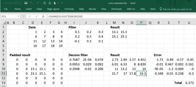
Here is a convolution. We start, let's say, with a 4 by 4 grid cell with a single channel. Let's put it through a 3 by 3 kernel with a single output filter. So we have a single channel in, a single filter kernel, so if we don't add any padding, we are going to end up with 2 by 2. Remember, the convolution is just the sum of the product of the kernel and the appropriate grid cell [1:11:09]. So there is our standard 3 by 3 conv one channel one filter.

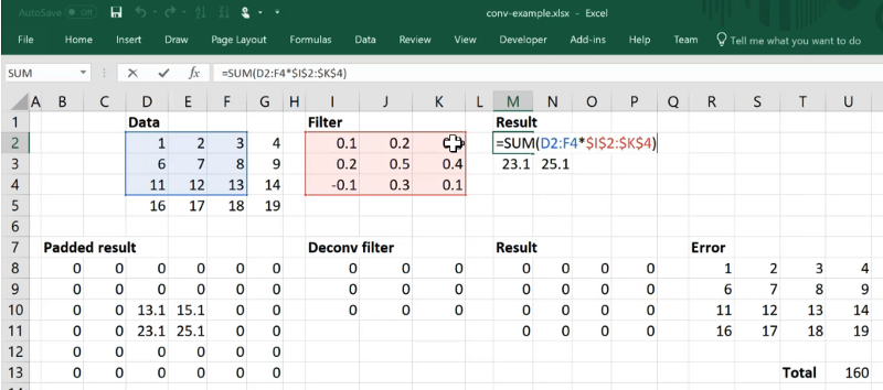
So the idea now is we want to go the opposite direction [1:11:25]. We want to start with our 2 by 2 and we want to create a 4 by 4. Specifically we want to create the same 4 by 4 that we started with. And we want to do that by using a convolution. How would we do that?

If we have a 3 by 3 convolution, then if we want to create a 4 by 4 output, we are going to need to create this much padding:

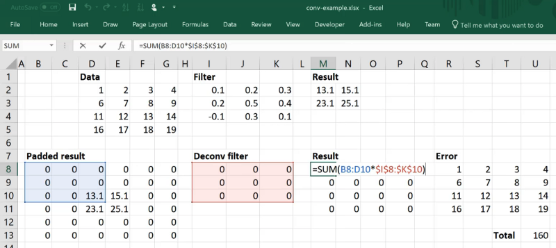
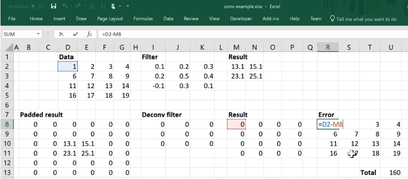
Because with this much padding, we are going to end up with 4 by 4. So let's say our convolutional filter was just a bunch of zeros then we can calculate our error for each cell just by taking this subtraction:

Then we can get the sum of absolute values (L1 loss) by summing up the absolute values of those errors:

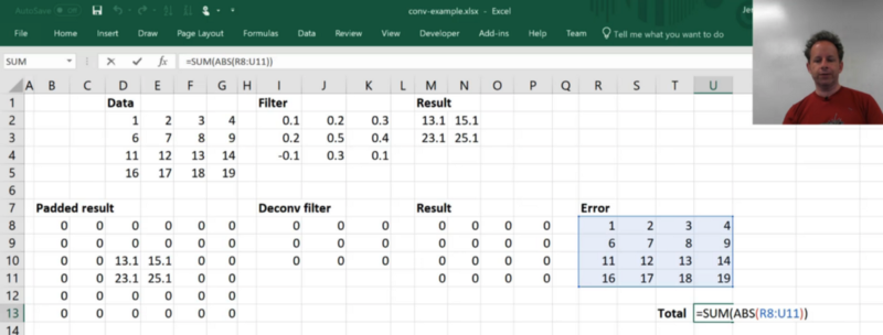
So now we could use optimization, in Excel it's called "solver" to do a gradient descent. So we will set the Total cell equal to minimum and we'll try and reduce our loss by changing our filter. You can see it's come up with a filter such that Result is almost like Data. It's not perfect, and in general, you can't assume that a deconvolution can exactly create the same exact thing you want because there is just not enough. Because there is 9 things in the filter and 16 things in the result. But it's made a pretty good attempt. So this is what a deconvolution looks like — a stride 1, 3x3 deconvolution on a 2x2 grid cell input.

❓ How difficult is it to create a discriminator to identify fake news vs. real news [1:13:43]?

You don't need anything special — that's just a classifier. So you would just use the NLP classifier from previous class and lesson 4. In that case, there is no generative piece, so you just need a dataset that says these are the things that we believe are fake news and these are the things we consider to be real news and it should actually work very well. To the best of our knowledge, if you try it you should get as good a result as anybody else has got — whether it's good enough to be useful in practice, Jeremy doesn't know. The best thing you could do at this stage would be to generate a kind of a triage that says these things look pretty sketchy based on how they are written and then some human could go in and fact check them. NLP classifier and RNN can't fact-check things but it could recognize that these are written in that kind of highly popularized style which often fake news is written in so maybe these ones are worth paying attention to. That would probably be the best you could hope for without drawing on some kind of external data sources. But it's important to remember the discriminator is basically just a classifier and you don't need any special techniques beyond what we've already learned to do NLP classification.

`ConvTranspose2d` [1:16:00]

To do deconvolution in PyTorch, just say:

nn.ConvTranspose2d(ni, no, ks, stride, padding=pad, bias=False)

ni : number of input channels
no: number of output channels
ks: kernel size

The reason it's called a ConvTranspose is because it turns out that this is the same as the calculation of the gradient of convolution. That's why they call it that.

Visualizing [1:16:33]

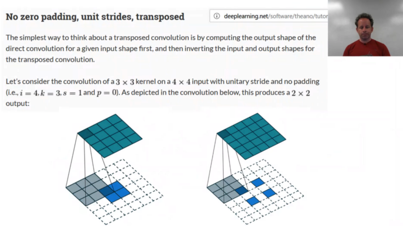
One on the left is what we just saw of doing a 2x2 deconvolution. If there is a stride 2, then you don't just have padding around the outside, but you actually have to put padding in the middle as well. They are not actually quite implemented this way because this is slow to do. In practice, you'll implement them in a different way but it all happens behind the scene, so you don't have to worry about it. We've talked about this convolution arithmetic tutorial before and if you are still not comfortable with convolutions and in order to get comfortable with deconvolutions, this is a great site to go to. If you want to see the paper, it is A guide to convolution arithmetic for deep learning.

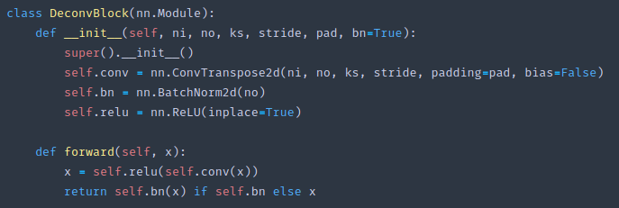
DeconvBlock looks identical to a ConvBlock except it has the word Transpose [1:17:49]. We just go conv → relu → batch norm as before, and it has input filters and output filters. The only difference is that stride 2 means that the grid size will double rather than half.

❓ Both nn.ConvTranspose2d and nn.Upsample seem to do the same thing, i.e. expand grid-size (height and width) from previous layer. Can we say nn.ConvTranspose2d is always better than nn.Upsample, since nn.Upsample is merely resize and fill unknowns by zero's or interpolation [1:18:10]?

No, you can't. There is a fantastic interactive paper on distill.pub called Deconvolution and Checkerboard Artifacts which points out that what we are doing right now is extremely suboptimal but the good news is everybody else does it.

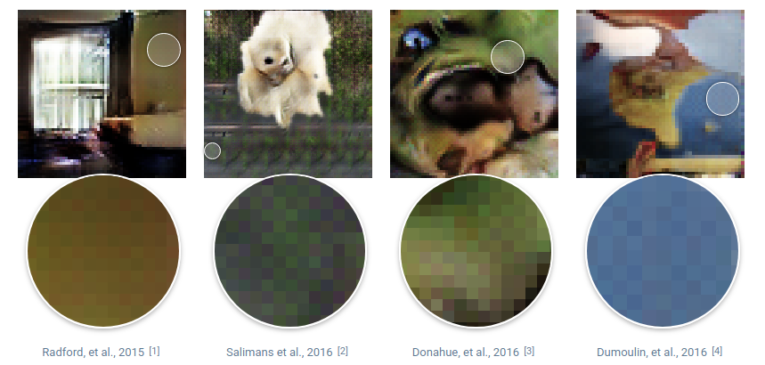
Have a look here, could you see these checkerboard artifacts? These are all from actual papers and basically they noticed every one of these papers with generative models have these checkerboard artifacts and what they realized is it's because when you have a stride 2 convolution of size three kernel, they overlap. So some grid cells gets twice as much activation.

So even if you start with random weights, you end up with a checkerboard artifacts. So deeper you get, the worse it gets. Their advice is less direct than it ought to be, Jeremy found that for most generative models, upsampling is better. If you nn.Upsample, it's basically doing the opposite of pooling — it says let's replace this one grid cell with four (2x2). There is a number of ways to upsample — one is just to copy it all across to those four, and other is to use bilinear or bicubic interpolation. There are various techniques to try and create a smooth upsampled version and you can choose any of them in PyTorch. If you do a 2 x 2 upsample and then regular stride one 3 x 3 convolution, that is another way of doing the same kind of thing as a ConvTranspose — it's doubling the grid size and doing some convolutional arithmetic on it. For generative models, it pretty much always works better. In that distil.pub publication, they indicate that maybe that's a good approach but they don't just come out and say just do this whereas Jeremy would just say just do this. Having said that, for GANS, he hasn't had that much success with it yet and he thinks it probably requires some tweaking to get it to work, The issue is that in the early stages, it doesn't create enough noise. He had a version where he tried to do it with an upsample and you could kind of see that the noise didn't look very noisy. Next week when we look at style transfer and super-resolution, you will see nn.Upsample really comes into its own.

The generator, we can now start with the vector [1:22:04]. We can decide and say okay let's not think of it as a vector but actually it's 1x1 grid cell, and then we can turn it into a 4x4 then 8x8 and so forth. That is why we have to make sure it's a suitable multiple so that we can create something of the right size. As you can see, it's doing the exact opposite as before. It's making the cell size bigger and bigger by 2 at a time as long as it can until it gets to half the size that we want, and then finally we add n more on at the end with stride 1. Then we add one more ConvTranspose to finally get to the size that we wanted and we are done. Finally we put that through a tanh and that will force us to be in the zero to one range because of course we don't want to spit out arbitrary size pixel values. So we have a generator architecture which spits out an image of some given size with the correct number of channels with values between zero and one.

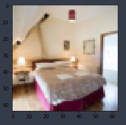
At this point, we can now create our model data object [1:23:38]. These things take a while to train, so we made it 128 by 128 (just a convenient way to make it a little bit faster). So that is going to be the size of the input, but then we are going to use transformation to turn it into 64 by 64.

There's been more recent advances which have attempted to really increase this up to high resolution sizes but they still tend to require either a batch size of 1 or lots and lots of GPUs [1:24:05]. So we are trying to do things that we can do with a single consumer GPU. Here is an example of one of the 64 by 64 bedrooms.

bs, sz, nz = 64, 64, 100

tfms = tfms_from_stats(inception_stats, sz)
md = ImageClassifierData.from_csv(PATH, 'bedroom', CSV_PATH, tfms=tfms, bs=128,
                                  skip_header=False, continuous=True)

md = md.resize(128)

x, _ = next(iter(md.val_dl))
plt.imshow(md.trn_ds.denorm(x)[0])

Putting them all together [1:24:30]

We are going to do pretty much everything manually so let's go ahead and create our two models — our generator and discriminator and as you can see they are DCGAN, so in other words, they are the same modules that appeared in this paper. It is well worth going back and looking at the DCGAN paper to see what these architectures are because it's assumed that when you read the Wasserstein GAN paper that you already know that.

netG = DCGAN_G(sz, nz, 3, 64, 1).cuda()
netD = DCGAN_D(sz, 3, 64, 1).cuda()

❓ Shouldn't we use a sigmoid if we want values between 0 and 1 [1:25:06]?

As usual, our images have been normalized to have a range from -1 to 1, so their pixel values don't go between 0 and 1 anymore. This is why we want values going from -1 to 1 otherwise we wouldn't give a correct input for the discriminator (via this post).

So we have a generator and a discriminator, and we need a function that returns a "prior" vector (i.e. a bunch of noise) [1:25:49]. We do that by creating a bunch of zeros. nz is the size of z —very often in our code, if you see a mysterious letter, it's because that's the letter they used in the paper. Here, z is the size of our noise vector. We then use normal distribution to generate random numbers between 0 and 1. And that needs to be a variable because it's going to be participating in the gradient updates.

def create_noise(b):
    return V(torch.zeros(b, nz, 1, 1).normal_(0, 1))

preds = netG(create_noise(4))
pred_ims = md.trn_ds.denorm(preds)

fig, axes = plt.subplots(2, 2, figsize=(6, 6))
for i, ax in enumerate(axes.flat):
    ax.imshow(pred_ims[i])

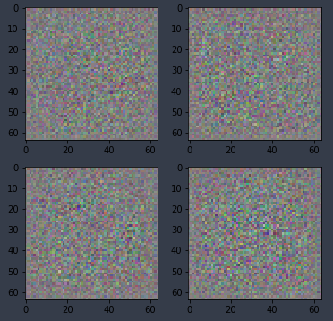
So here is an example of creating some noise and resulting four different pieces of noise.

def gallery(x, nc=3):
    n, h, w, c = x.shape
    nr = n // nc
    assert n == nr * nc
    return (x.reshape(nr, nc, h, w, c)
               .swapaxes(1, 2)
               .reshape(h * nr, w * nc, c))

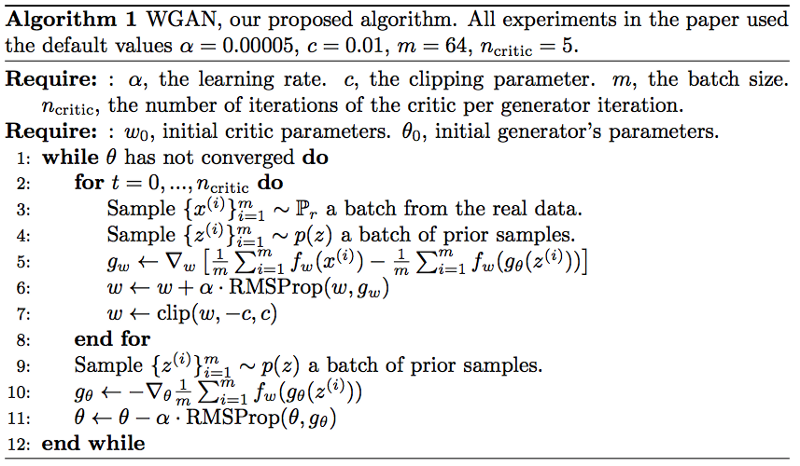
We need an optimizer in order to update our gradients [1:26:41]. In the Wasserstein GAN paper, they told us to use RMSProp:

We can easily do that in PyTorch:

optimizerD = optim.RMSprop(netD.parameters(), lr=1e-4)
optimizerG = optim.RMSprop(netG.parameters(), lr=1e-4)

In the paper, they suggested a learning rate of 0.00005 (5e-5), we found 1e-4 seem to work, so we made it a little bit bigger.

Now we need a training loop [1:27:14]:

def train(niter, first=True):
    gen_iterations = 0
    for epoch in trange(niter):
        netD.train()
        netG.train()
        data_iter = iter(md.trn_dl)
        i, n = 0,len(md.trn_dl)
        with tqdm(total=n) as pbar:
            while i < n:
                set_trainable(netD, True)
                set_trainable(netG, False)
                d_iters = 100 if (first and (gen_iterations < 25) or (gen_iterations % 500 == 0)) else 5
                j = 0
                while (j < d_iters) and (i < n):
                    j += 1
                    i += 1
                    for p in netD.parameters():
                        p.data.clamp_(-0.01, 0.01)
                    real = V(next(data_iter)[0])
                    real_loss = netD(real)
                    fake = netG(create_noise(real.size(0)))
                    fake_loss = netD(V(fake.data))
                    netD.zero_grad()
                    lossD = real_loss - fake_loss
                    lossD.backward()
                    optimizerD.step()
                    pbar.update()

                set_trainable(netD, False)
                set_trainable(netG, True)
                netG.zero_grad()
                lossG = netD(netG(create_noise(bs))).mean(0).view(1)
                lossG.backward()
                optimizerG.step()
                gen_iterations += 1

        print(f'Loss_D {to_np(lossD)}; Loss_G {to_np(lossG)}; '
              f'D_real {to_np(real_loss)}; Loss_D_fake {to_np(fake_loss)}')

A training loop will go through some number of epochs that we get to pick (so that's going to be a parameter). Remember, when you do everything manually, you've got to remember all the manual steps to do:

You have to set your modules into training mode when you are training them and into evaluation mode when you are evaluating because in training mode batch norm updates happen and dropout happens, in evaluation mode, those two things gets turned off.
We are going to grab an iterator from our training data loader
We are going to see how many steps we have to go through and then we will use tqdm to give us a progress bar, and we are going to go through that many steps.

The first step of the algorithm in the paper is to update the discriminator (in the paper, they call discriminator a "critic" and w is the weights of the critic). So the first step is to train our critic a little bit, and then we are going to train our generator a little bit, and we will go back to the top of the loop. The inner for loop in the paper correspond to the second while loop in our code.

What we are going to do now is we have a generator that is random at the moment [1:29:06]. So our generator will generate something that looks like the noise. First of all, we need to teach our discriminator to tell the difference between the noise and a bedroom — which shouldn't be too hard you would hope. So we just do it in the usual way but there is a few little tweaks:

We are going to grab a mini batch of real bedroom photos so we can just grab the next batch from our iterator, turn it into a variable.
Then we are going to calculate the loss for that — so this is going to be how much the discriminator thinks this looks fake ("does the real one look fake?").
Then we are going to create some fake images and to do that we will create some random noise, and we will stick it through our generator which at this stage is just a bunch of random weights. That will create a mini batch of fake images.
Then we will put that through the same discriminator module as before to get the loss for that ("how fake does the fake one look?"). Remember, when you do everything manually, you have to zero the gradients (netD.zero_grad()) in your loop. If you have forgotten about that, go back to the part 1 lesson where we do everything from scratch.
Finally, the total discriminator loss is equal to the real loss minus the fake loss.

So you can see that here [1:30:58]:

They don't talk about the loss, they actually just talk about one of the gradient updates.

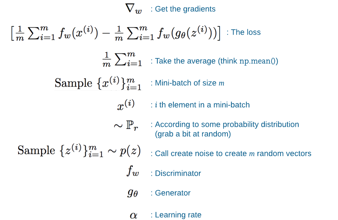
In PyTorch, we don't have to worry about getting the gradients, we can just specify the loss and call loss.backward() then discriminator's optimizer.step() [1:34:27]. There is one key step which is that we have to keep all of our weights which are the parameters in PyTorch module in the small range of -0.01 and 0.01. Why? Because the mathematical assumptions that make this algorithm work only apply in a small ball. It is interesting to understand the math of why that is the case, but it's very specific to this one paper and understanding it won't help you understand any other paper, so only study it if you are interested. It is nicely explained and Jeremy thinks it's fun but it won't be information that you will reuse elsewhere unless you get super into GANs. He also mentioned that after the paper came out, an improved Wasserstein GAN came out that said there are better ways to ensure that your weight space is in this tight ball which was to penalize gradients that are too high, so nowadays there are slightly different ways to do this. But this line of code is the key contribution and it is what makes it Wasserstein GAN:

for p in netD.parameters():
    p.data.clamp_(-0.01, 0.01)

At the end of this, we have a discriminator that can recognize real bedrooms and our totally random crappy generated images [1:36:20]. Let's now try and create some better images. So now set trainable discriminator to false, set trainable generator to true, zero out the gradients of the generator. Our loss again is fw (discriminator) of the generator applied to some more random noise. So it's exactly the same as before where we did generator on the noise and then pass that to a discriminator, but this time, the thing that's trainable is the generator, not the discriminator. In other words, in the pseudo code, the thing they update is Ɵ which is the generator's parameters. So it takes noise, generate some images, try and figure out if they are fake or real, and use that to get gradients with respect to the generator, as opposed to earlier we got them with respect to the discriminator, and use that to update our weights with RMSProp with an alpha learning rate [1:38:21].

You'll see that it's unfair that the discriminator is getting trained ncritic times (d_iters in above code) which they set to 5 for every time we train the generator once. And the paper talks a bit about this but the basic idea is there is no point making the generator better if the discriminator doesn't know how to discriminate yet. So that's why we have the second while loop. And here is that 5:

d_iters = 100 if (first and (gen_iterations < 25) or (gen_iterations % 500 == 0)) else 5

Actually something which was added in the later paper or maybe supplementary material is the idea that from time to time and a bunch of times at the start, you should do more steps at the discriminator to make sure that the discriminator is capable.

torch.backends.cudnn.benchmark = True

Let's train that for one epoch:

train(1, False)

# -----------------------------------------------------------------------------
# Output
# -----------------------------------------------------------------------------
100%|██████████| 1900/1900 [08:28<00:00,  1.75it/s]
Loss_D [-0.78008]; Loss_G [-0.33545]; D_real [-0.16079]; Loss_D_fake [0.61929]
100%|██████████| 1/1 [08:28<00:00, 508.58s/it]

Then let's create some noise so we can generate some examples.

fixed_noise = create_noise(bs)

But before that, reduce the learning rate by 10 and do one more pass:

set_trainable(netD, True)
set_trainable(netG, True)
optimizerD = optim.RMSprop(netD.parameters(), lr=1e-5)
optimizerG = optim.RMSprop(netG.parameters(), lr=1e-5)

train(1, False)

# -----------------------------------------------------------------------------
# Output
# -----------------------------------------------------------------------------
100%|██████████| 1900/1900 [08:17<00:00,  4.01it/s]
Loss_D [-1.42976]; Loss_G [0.70786]; D_real [-0.70362]; Loss_D_fake [0.72613]
100%|██████████| 1/1 [08:17<00:00, 497.96s/it]

Then let's use the noise to pass it to our generator, then put it through our denormalization to turn it back into something we can see, and then plot it:

netD.eval()
netG.eval()
fake = netG(fixed_noise).data.cpu()
faked = np.clip(md.trn_ds.denorm(fake), 0, 1)

plt.figure(figsize=(9, 9))
plt.imshow(gallery(faked, 8))

# Save our work
def save_state(net, fn):
    torch.save(net.state_dict(), TMP_PATH / fn)

save_state(netG, 'netG_full_data.h5') # save generator
save_state(netD, 'netD_full_data.h5') # save discriminator

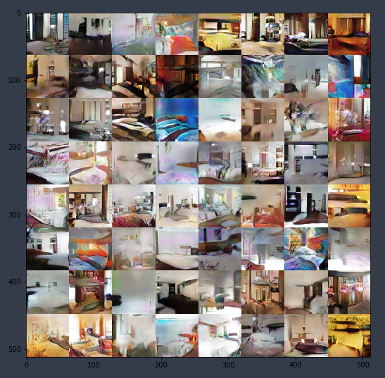
Generated images of training using the full data:

Generated images of training using the sample data:

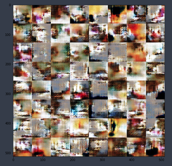
These are results of training using the sample data, a random 10% of our dataset and full data. ~~We will try experimenting using the full dataset.~~

And we have some bedrooms. These are not real bedrooms, and some of them don't look particularly like bedrooms, but some of them look a lot like bedrooms, so that's the idea. That's GAN. The best way to think about GAN is it is like an underlying technology that you will probably never use like this, but you will use in lots of interesting ways. For example, we are going to use it to create a cycle GAN.

❓ Is there any reason for using RMSProp specifically as the optimizer as opposed to Adam etc. [1:41:38]?

I don't remember it being explicitly discussed in the paper. I don't know if it's just experimental or the theoretical reason. Have a look in the paper and see what it says.

From the forum

From experimenting I figured that Adam and WGANs not just work worse — it causes to completely fail to train meaningful generator.
from WGAN paper:
Finally, as a negative result, we report that WGAN training becomes unstable at times when one uses a momentum based optimizer such as Adam [8] (with β1>0) on the critic, or when one uses high learning rates. Since the loss for the critic is nonstationary, momentum based methods seemed to perform worse. We identified momentum as a potential cause because, as the loss blew up and samples got worse, the cosine between the Adam step and the gradient usually turned negative. The only places where this cosine was negative was in these situations of instability. We therefore switched to RMSProp [21] which is known to perform well even on very nonstationary problems.

❓ Which could be a reasonable way of detecting overfitting while training? Or of evaluating the performance of one of these GAN models once we are done training? In other words, how does the notion of train/val/test sets translate to GANs [1:41:57]?

That is an awesome question, and there's a lot of people who make jokes about how GANs is the one field where you don't need a test set and people take advantage of that by making stuff up and saying it looks great. There are some famous problems with GANs, one of them is called Mode Collapse. Mode collapse happens where you look at your bedrooms and it turns out that there's only three kinds of bedrooms that every possible noise vector maps to. You look at your gallery and it turns out they are all just the same thing or just three different things. Mode collapse is easy to see if you collapse down to a small number of modes, like 3 or 4. But what if you have a mode collapse down to 10,000 modes? So there are only 10,000 possible bedrooms that all of your noise vectors collapse to. You wouldn't be able to see in the gallery view we just saw because it's unlikely you would have two identical bedrooms out of 10,000. Or what if every one of these bedrooms is basically a direct copy of one of the input — it basically memorized some input. Could that be happening? And the truth is, most papers don't do a good job or sometimes any job of checking those things. So the question of how do we evaluate GANS and even the point of maybe we should actually evaluate GANs properly is something that is not widely enough understood even now. Some people are trying to really push. Ian Goodfellow was the first author on the most famous deep learning book and is the inventor of GANs and he's been sending continuous stream of tweets reminding people about the importance of testing GANs properly. If you see a paper that claims exceptional GAN results, then this is definitely something to look at. Have they talked about mode collapse? Have they talked about memorization? And so forth.

❓ Can GANs be used for data augmentation [1:45:33]?

Yeah, absolutely you can use GAN for data augmentation. Should you? I don't know. There are some papers that try to do semi-supervised learning with GANs. I haven't found any that are particularly compelling showing state-of-the-art results on really interesting datasets that have been widely studied. I'm a little skeptical and the reason I'm a little skeptical is because in my experience, if you train a model with synthetic data, the neural net will become fantastically good at recognizing the specific problems of your synthetic data and that'll end up what it's learning from. There are lots of other ways of doing semi-supervised models which do work well. There are some places that can work. For example, you might remember Otavio Good created that fantastic visualization in part 1 of the zooming conv net where it showed letter going through MNIST, he, at least at that time, was the number one in autonomous remote control car competitions, and he trained his model using synthetically augmented data where he basically took real videos of a car driving around the circuit and added fake people and fake other cars. I think that worked well because A. he is kind of a genius and B. because I think he had a well defined little subset that he had to work in. But in general, it's really really hard to use synthetic data. I've tried using synthetic data and models for decades now (obviously not GANs because they're pretty new) but in general it's very hard to do. Very interesting research question.

⭐ ⭐ More Wasserstein GAN experiments from me in my GitHub repo ⭐ ⭐

Cycle GAN [1:41:08]

We are going to use Cycle GAN to turn horses into zebras. You can also use it to turn Monet prints into photos or to turn photos of Yosemite in summer into winter.

This is going to be really straight forward because it's just a neural net [1:44:46]. All we are going to do is we are going to create an input containing lots of zebra photos and with each one we'll pair it with an equivalent horse photo and we'll just train a neural net that goes from one to the other. Or you could do the same thing for every Monet painting — create a dataset containing the photo of the place …oh wait, that's not possible because the places that Monet painted aren't there anymore and there aren't exact zebra versions of horses …how the heck is this going to work? This seems to break everything we know about what neural nets can do and how they do them.

So somehow these folks at Berkeley cerated a model that can turn a horse into a zebra despite not having any photos. Unless they went out there and painted horses and took before-and-after shots but I believe they didn't [1:47:51]. So how the heck did they do this? It's kind of genius.

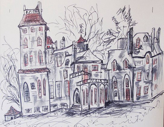
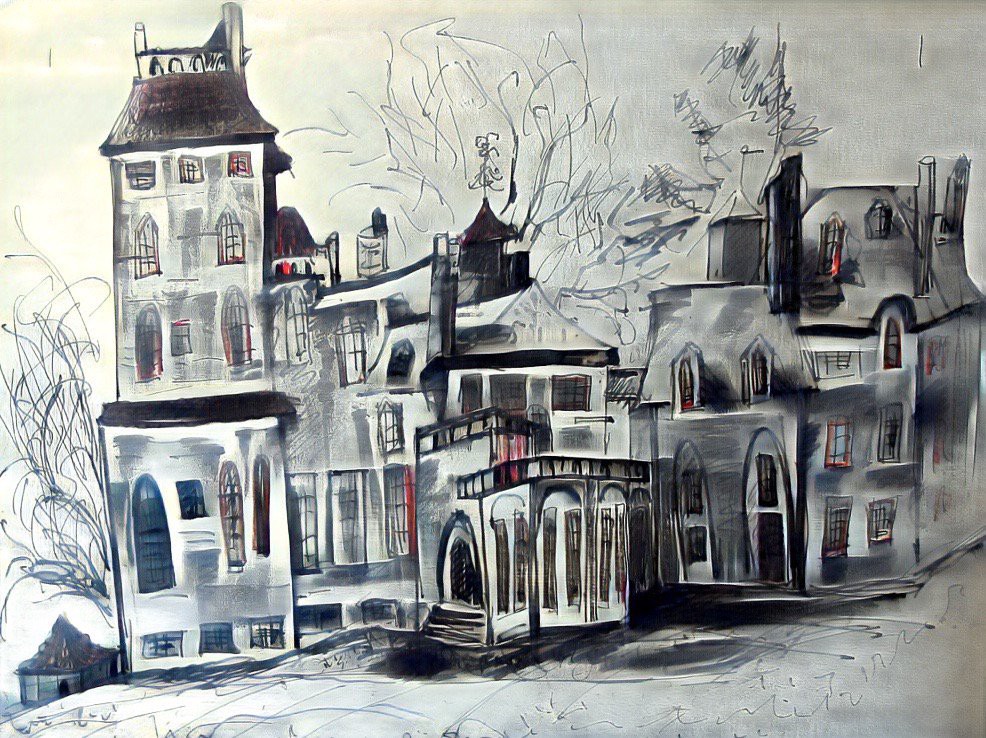
The person I know who is doing the most interesting practice of Cycle GAN right now is one of our students Helena Sarin @glagolista. She is the only artist I know of who is a Cycle GAN artist.

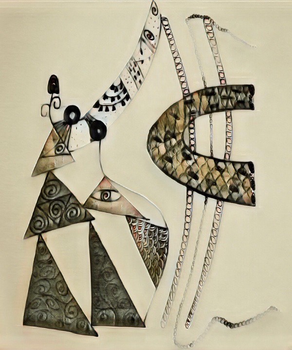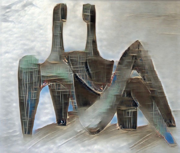Here are some more of her amazing works and I think it's really interesting. I mentioned at the start of this class that GANs are in the category of stuff that is not there yet, but it's nearly there. And in this case, there is at least one person in the world who is creating beautiful and extraordinary artworks using GANs (specifically Cycle GANs). At least a dozen people I know of who are just doing interesting creative work with neural nets more generally. And the field of creative AI is going to expand dramatically.

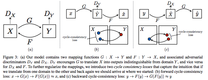
Here is the basic trick [1:50:11]. This is from the Cycle GAN paper. We are going to have two images (assuming we are doing this with images). The key thing is they are not paired images, so we don't have a dataset of horses and the equivalent zebras. We have bunch of horses, and bunch of zebras. Grab one horse X, grab one zebra Y. We are going to train a generator (what they call here a "mapping function") that turns horse into zebra. We'll call that mapping function G and we'll create one mapping function (a.k.a. generator) that turns a zebra into a horse and we will call that F. We will create a discriminator just like we did before which is going to get as good as possible at recognizing real from fake horses so that will be Dx. Another discriminator which is going to be as good as possible at recognizing real from fake zebras, we will call that Dy. That is our starting point.

The key thing to making this work [1:51:27]—so we are generating a loss function here (Dx and Dy). We are going to create something called cycle-consistency loss which says after you turn your horse into a zebra with your generator, and check whether or not I can recognize that it's a real. We turn our horse into a zebra and then going to try and turn that zebra back into the same horse that we started with. Then we are going to have another function that is going to check whether this horse which are generated knowing nothing about x — generated entirely from this zebra Y is similar to the original horse or not. So the idea would be if your generated zebra doesn't look anything like your original horse, you've got no chance of turning it back into the original horse. So a loss which compares x-hat to x is going to be really bad unless you can go into Y and back out again and you're probably going to be able to do that if you're able to create a zebra that looks like the original horse so that you know what the original horse looked like. And vice versa — take your zebra, turn it into a fake horse, and check that you can recognize that and then try and turn it back into the original zebra and check that it looks like the original.

So notice F (zebra to horse) and G (horse to zebra) are doing two things [1:53:09]. They are both turning the original horse into the zebra, and then turning the zebra back into the original horse. So there are only two generators. There isn't a separate generator for the reverse mapping. You have to use the same generator that was used for the original mapping. So this is the cycle-consistency loss. I think this is genius. The idea that this is a thing that could even be possible. Honestly when this came out, it just never occurred to me as a thing that I could even try and solve. It seems so obviously impossible and then the idea that you can solve it like this — I just think it's so darn smart.

It's good to look at the equations in this paper because they are good examples — they are written pretty simply and it's not like some of the Wasserstein GAN paper which is lots of theoretical proofs and whatever else [1:54:05]. In this case, they are just equations that lay out what's going on. You really want to get to a point where you can read them and understand them.

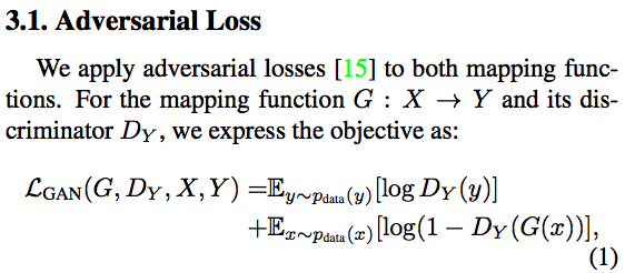
So we've got a horse X and a zebra Y [1:54:34]. For some mapping function G which is our horse to zebra mapping function, then there is a GAN loss which is a bit we are already familiar with it says we have a horse, a zebra, a fake zebra recognizer, and a horse-zebra generator. The loss is what we saw before — it's our ability to draw one zebra out of our zebras and recognize whether it is real or fake. Then take a horse and turn it into a zebra and recognize whether that's real or fake. You then do one minus the other (in this case, they have a log in there but the log is not terribly important). So this is the thing we just saw. That is why we did Wasserstein GAN first. This is just a standard GAN loss in math form.

❓ All of this sounds awfully like translating in one language to another then back to the original. Have GANs or any equivalent been tried in translation [1:55:54]?

Paper from the forum. Back up to what I do know — normally with translation you require this kind of paired input (i.e. parallel text — "this is the French translation of this English sentence"). There has been a couple of recent papers that show the ability to create good quality translation models without paired data.

🔖 I haven't implemented them and I don't understand anything I haven't implemented, but they may well be doing the same basic idea. We'll look at it during the week and get back to you.

Cycle-consistency loss [1:57:14]

So we've got a GAN loss and the next piece is the cycle-consistency loss. So the basic idea here is that we start with our horse, use our zebra generator on that to create a zebra, use our horse generator on that to create a horse and compare that to the original horse. This double lines with the 1 is the L1 loss — sum of the absolute value of differences [1:57:35]. Where else if this was 2, it would be the L2 loss so the 2-norm which would be the sum of the squared differences.

We now know this squiggle idea which is from our horses grab a horse. This is what we mean by sample from a distribution. There's all kinds of distributions but most commonly in these papers we're using an empirical distribution, in other words we've got some rows of data, grab a row. So here, it is saying grab something from the data and we are going to call that thing x. To recapture:

From our horse pictures, grab a horse
Turn it into a zebra
Turn it back into a horse
Compare it to the original and sum of the absolute values
Do it for zebra to horse as well
And add the two together

That is our cycle-consistency loss.

Full objective [1:58:54]

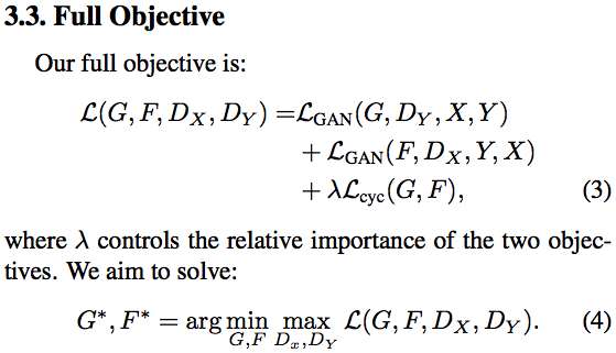
Now we get our loss function and the whole loss function depends on:

our horse generator
a zebra generator
our horse recognizer
our zebra recognizer (a.k.a. discriminator)

We are going to add up:

the GAN loss for recognizing horses
GAN loss for recognizing zebras
the cycle-consistency loss for our two generators

We have a lambda here which hopefully we are kind of used to this idea now that is when you have two different kinds of loss, you chuck in a parameter there you can multiply them by so they are about the same scale [1:59:23]. We did a similar thing with our bounding box loss compared to our classifier loss when we did the localization.

Then for this loss function, we are going to try to maximize the capability of the discriminators to discriminate, whilst minimizing that for the generators. So the generators and the discriminators are going to be facing off against each other. When you see this min max thing in papers, it basically means this idea that in your training loop, one thing is trying to make something better, the other is trying to make something worse, and there're lots of ways to do it but most commonly, you'll alternate between the two. You will often see this just referred to in math papers as min-max. So when you see min-max, you should immediately think adversarial training.

Implementing Cycle GAN [2:00:41]

Let's look at the code. We are going to do something almost unheard of which is I started looking at somebody else's code and I was not so disgusted that I threw the whole thing away and did it myself. I actually said I quite like this, I like it enough I'm going to show it to my students. This is where the code came from, and this is one of the people that created the original code for Cycle GANs and they created a PyTorch version. I had to clean it up a little bit but it's actually pretty darn good. The cool thing about this is that you are now going to get to see almost all the bits of fast.ai or all the relevant bits of fast.ai written in a different way by somebody else. So you're going to get to see how they do datasets, data loaders, models, training loops, and so forth.

You'll find there is a cgan directory [2:02:12] which is basically nearly the original with some cleanups which I hope to submit as a PR sometime. It was written in a way that unfortunately made it a bit over connected to how they were using it as a script, so I cleaned it up a little bit so I could use it as a module. But other than that, it's pretty similar.

from fastai.conv_learner import *
from fastai.dataset import *
from cgan.options.train_options import *

So cgan is their code copied from their GitHub repo with some minor changes. The way cgan mini library has been set up is that the configuration options, they are assuming, are being passed into like a script. So they have TrainOptions().parse method and I'm basically passing in an array of script options (where's my data, how many threads, do I want to dropout, how many iterations, what am I going to call this model, which GPU do I want run it on). That gives us an opt object which you can see what it contains. You'll see that it contains some things we didn't mention that is because it has defaults for everything else that we didn't mention.

opt = TrainOptions().parse(['--dataroot', 'cgan/datasets/horse2zebra', '--nThreads', '8', '--no_dropout',
                           '--niter', '100', '--niter_decay', '100', '--name', 'nodrop', '--gpu_ids', '0'])

# -----------------------------------------------------------------------------
# Output
# -----------------------------------------------------------------------------
------------ Options -------------
: 0.5
checkpoints_dir: ./checkpoints
continue_train: False
dataroot: cgan/datasets/horse2zebra
dataset_mode: unaligned
display_freq: 100
display_id: 1
display_port: 8097
display_single_pane_ncols: 0
display_winsize: 256
epoch_count: 1
fineSize: 256
gpu_ids: [0]
init_type: normal
input_nc: 3
isTrain: True
lambda_A: 10.0
lambda_B: 10.0
lambda_identity: 0.5
loadSize: 286
lr: 0.0002
lr_decay_iters: 50
lr_policy: lambda
max_dataset_size: inf
model: cycle_gan
nThreads: 8
n_layers_D: 3
name: nodrop
ndf: 64
ngf: 64
niter: 100
niter_decay: 100
no_dropout: True
no_flip: False
no_html: False
no_lsgan: False
norm: instance
output_nc: 3
phase: train
pool_size: 50
print_freq: 100
resize_or_crop: resize_and_crop
save_epoch_freq: 5
save_latest_freq: 5000
serial_batches: False
update_html_freq: 1000
which_direction: AtoB
which_epoch: latest
which_model_netD: basic
which_model_netG: resnet_9blocks
-------------- End ----------------

Download dataset

The original CycleGAN GitHub repo provides shell scripts to download the dataset: https://github.com/junyanz/pytorch-CycleGAN-and-pix2pix/blob/master/datasets/download_cyclegan_dataset.sh

You can download the 'horse2zebra' dataset file using this direct link if you prefer: https://people.eecs.berkeley.edu/~taesung_park/CycleGAN/datasets/horse2zebra.zip

%cd cgan/

!bash ./datasets/download_cyclegan_dataset.sh horse2zebra

--2018-07-10 10:21:26--  https://people.eecs.berkeley.edu/~taesung_park/CycleGAN/datasets/horse2zebra.zip
Resolving people.eecs.berkeley.edu (people.eecs.berkeley.edu)... 128.32.189.73
Connecting to people.eecs.berkeley.edu (people.eecs.berkeley.edu)|128.32.189.73|:443... connected.
HTTP request sent, awaiting response... 200 OK
Length: 116867962 (111M) [application/zip]
Saving to: ‘./datasets/horse2zebra.zip'

./datasets/horse2ze 100%[===================>] 111.45M  11.1MB/s    in 11s

2018-07-10 10:21:38 (10.3 MB/s) - ‘./datasets/horse2zebra.zip' saved [116867962/116867962]

Archive:  ./datasets/horse2zebra.zip
   creating: ./datasets/horse2zebra/trainA/
  inflating: ./datasets/horse2zebra/trainA/n02381460_6223.jpg
  inflating: ./datasets/horse2zebra/trainA/n02381460_1567.jpg
  ... ... ... ... ... ...
  ... ... ... ... ... ...
  inflating: ./datasets/horse2zebra/testA/n02381460_7970.jpg

%cd ..

Data loader

So rather than using fast.ai stuff, we are going to largely use cgan stuff.

from cgan.data.data_loader import CreateDataLoader
from cgan.models.models import create_model

The first thing we are going to need is a data loader. So this is also a great opportunity for you again to practice your ability to navigate through code with your editor or IDE of choice. We are going to start with CreateDataLoader. You should be able to go find symbol or in vim tag to jump straight to CreateDataLoader and we can see that's creating a CustomDatasetDataLoader. Then we can see CustomDatasetDataLoader is a BaseDataLoader. We can see that it's going to use a standard PyTorch DataLoader, so that's good. We know if you are going to use a standard PyTorch DataLoader, you have pass it a dataset, and we know that a dataset is something that contains a length and an indexer so presumably when we look at CreateDataset it's going to do that.

Here is CreateDataset and this library does more than just Cycle GAN — it handles both aligned and unaligned image pairs [2:04:46]. We know that our image pairs are unaligned so we are going to UnalignedDataset.

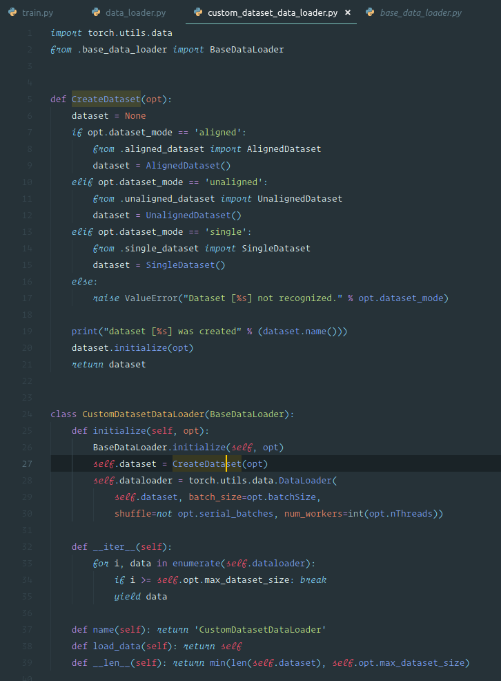
As expected, it has __getitem__ and __len__. For length, A and B are our horses and zebras, we got two sets, so whichever one is longer is the length of the DataLoader. __getitem__ is going to:

Randomly grab something from each of our two horses and zebras
Open them up with pillow (PIL)
Run them through some transformations
Then we could either be turning horses into zebras or zebras into horses, so there's some direction
Return our horse, zebra, a path to the horse, and a path of zebra

Hopefully you can kind of see that this is looking pretty similar to the kind of things fast.ai does. Fast.ai obviously does quite a lot more when it comes to transforms and performance, but remember, this is research code for this one thing and it's pretty cool that they did all this work.

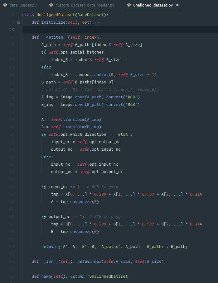
data_loader = CreateDataLoader(opt)
dataset = data_loader.load_data()
dataset_size = len(data_loader)
dataset_size

# -----------------------------------------------------------------------------
# Output
# -----------------------------------------------------------------------------
CustomDatasetDataLoader
dataset [UnalignedDataset] was created
1334

We've got a data loader so we can go and load our data into it [2:06:17]. That will tell us how many mini-batches are in it (that's the length of the data loader in PyTorch).

Next step is to create a model. Same idea, we've got different kind of models and we're going to be doing a Cycle GAN.

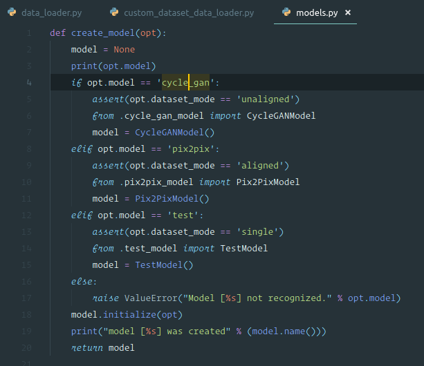
Here is our CycleGANModel. There is quite a lot of stuff in CycleGANModel, so let's go through and find out what's going to be used. At this stage, we've just called initializer so when we initialize it, it's going to go through and define two generators which is not surprising a generator for our horses and a generator for zebras. There is some way for it to generate a pool of fake data and then we're going to grab our GAN loss, and as we talked about our cycle-consistency loss is an L1 loss. They are going to use Adam, so obviously for Cycle GANS they found Adam works pretty well. Then we are going to have an optimizer for our horse discriminator, an optimizer for our zebra discriminator, and an optimizer for our generator. The optimizer for the generator is going to contain the parameters both for the horse generator and the zebra generator all in one place.

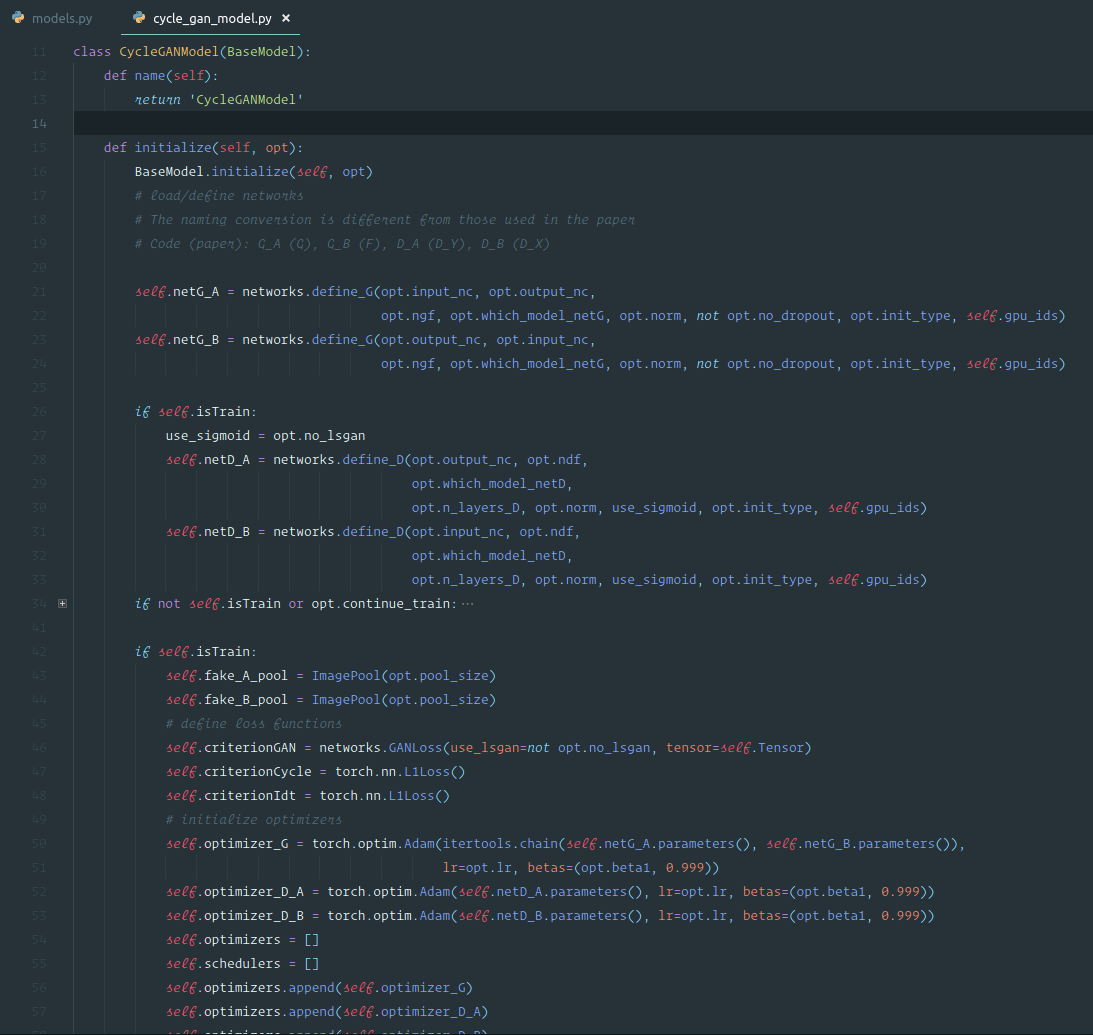
So the initializer is going to set up all of the different networks and loss functions we need and they are going to be stored inside this model [2:08:14].

model = create_model(opt)

# -----------------------------------------------------------------------------
# Output
# -----------------------------------------------------------------------------
cycle_gan
initialization method [normal]
initialization method [normal]
initialization method [normal]
initialization method [normal]
---------- Networks initialized -------------
ResnetGenerator(
  (model): Sequential(
    (0): ReflectionPad2d((3, 3, 3, 3))
    (1): Conv2d(3, 64, kernel_size=(7, 7), stride=(1, 1))
    (2): InstanceNorm2d(64, eps=1e-05, momentum=0.1, affine=False)
    (3): ReLU(inplace)
    (4): Conv2d(64, 128, kernel_size=(3, 3), stride=(2, 2), padding=(1, 1))
    (5): InstanceNorm2d(128, eps=1e-05, momentum=0.1, affine=False)
    (6): ReLU(inplace)
    (7): Conv2d(128, 256, kernel_size=(3, 3), stride=(2, 2), padding=(1, 1))
    (8): InstanceNorm2d(256, eps=1e-05, momentum=0.1, affine=False)
    (9): ReLU(inplace)
    (10): ResnetBlock(
      (conv_block): Sequential(
        (0): ReflectionPad2d((1, 1, 1, 1))
        (1): Conv2d(256, 256, kernel_size=(3, 3), stride=(1, 1))
        (2): InstanceNorm2d(256, eps=1e-05, momentum=0.1, affine=False)
        (3): ReLU(inplace)
        (4): ReflectionPad2d((1, 1, 1, 1))
        (5): Conv2d(256, 256, kernel_size=(3, 3), stride=(1, 1))
        (6): InstanceNorm2d(256, eps=1e-05, momentum=0.1, affine=False)
      )
    )

    ... ... ... trucated ... ... ...
    ... ... ... trucated ... ... ...

    (18): ResnetBlock(
      (conv_block): Sequential(
        (0): ReflectionPad2d((1, 1, 1, 1))
        (1): Conv2d(256, 256, kernel_size=(3, 3), stride=(1, 1))
        (2): InstanceNorm2d(256, eps=1e-05, momentum=0.1, affine=False)
        (3): ReLU(inplace)
        (4): ReflectionPad2d((1, 1, 1, 1))
        (5): Conv2d(256, 256, kernel_size=(3, 3), stride=(1, 1))
        (6): InstanceNorm2d(256, eps=1e-05, momentum=0.1, affine=False)
      )
    )
    (19): ConvTranspose2d(256, 128, kernel_size=(3, 3), stride=(2, 2), padding=(1, 1), output_padding=(1, 1))
    (20): InstanceNorm2d(128, eps=1e-05, momentum=0.1, affine=False)
    (21): ReLU(inplace)
    (22): ConvTranspose2d(128, 64, kernel_size=(3, 3), stride=(2, 2), padding=(1, 1), output_padding=(1, 1))
    (23): InstanceNorm2d(64, eps=1e-05, momentum=0.1, affine=False)
    (24): ReLU(inplace)
    (25): ReflectionPad2d((3, 3, 3, 3))
    (26): Conv2d(64, 3, kernel_size=(7, 7), stride=(1, 1))
    (27): Tanh()
  )
)
Total number of parameters: 11378179
ResnetGenerator(
  (model): Sequential(
    (0): ReflectionPad2d((3, 3, 3, 3))
    (1): Conv2d(3, 64, kernel_size=(7, 7), stride=(1, 1))
    (2): InstanceNorm2d(64, eps=1e-05, momentum=0.1, affine=False)
    (3): ReLU(inplace)
    (4): Conv2d(64, 128, kernel_size=(3, 3), stride=(2, 2), padding=(1, 1))
    (5): InstanceNorm2d(128, eps=1e-05, momentum=0.1, affine=False)
    (6): ReLU(inplace)
    (7): Conv2d(128, 256, kernel_size=(3, 3), stride=(2, 2), padding=(1, 1))
    (8): InstanceNorm2d(256, eps=1e-05, momentum=0.1, affine=False)
    (9): ReLU(inplace)
    (10): ResnetBlock(
      (conv_block): Sequential(
        (0): ReflectionPad2d((1, 1, 1, 1))
        (1): Conv2d(256, 256, kernel_size=(3, 3), stride=(1, 1))
        (2): InstanceNorm2d(256, eps=1e-05, momentum=0.1, affine=False)
        (3): ReLU(inplace)
        (4): ReflectionPad2d((1, 1, 1, 1))
        (5): Conv2d(256, 256, kernel_size=(3, 3), stride=(1, 1))
        (6): InstanceNorm2d(256, eps=1e-05, momentum=0.1, affine=False)
      )
    )
    (11): ResnetBlock(
      (conv_block): Sequential(
        (0): ReflectionPad2d((1, 1, 1, 1))
        (1): Conv2d(256, 256, kernel_size=(3, 3), stride=(1, 1))
        (2): InstanceNorm2d(256, eps=1e-05, momentum=0.1, affine=False)
        (3): ReLU(inplace)
        (4): ReflectionPad2d((1, 1, 1, 1))
        (5): Conv2d(256, 256, kernel_size=(3, 3), stride=(1, 1))
        (6): InstanceNorm2d(256, eps=1e-05, momentum=0.1, affine=False)
      )
    )

    ... ... ... trucated ... ... ...
    ... ... ... trucated ... ... ...

    (18): ResnetBlock(
      (conv_block): Sequential(
        (0): ReflectionPad2d((1, 1, 1, 1))
        (1): Conv2d(256, 256, kernel_size=(3, 3), stride=(1, 1))
        (2): InstanceNorm2d(256, eps=1e-05, momentum=0.1, affine=False)
        (3): ReLU(inplace)
        (4): ReflectionPad2d((1, 1, 1, 1))
        (5): Conv2d(256, 256, kernel_size=(3, 3), stride=(1, 1))
        (6): InstanceNorm2d(256, eps=1e-05, momentum=0.1, affine=False)
      )
    )
    (19): ConvTranspose2d(256, 128, kernel_size=(3, 3), stride=(2, 2), padding=(1, 1), output_padding=(1, 1))
    (20): InstanceNorm2d(128, eps=1e-05, momentum=0.1, affine=False)
    (21): ReLU(inplace)
    (22): ConvTranspose2d(128, 64, kernel_size=(3, 3), stride=(2, 2), padding=(1, 1), output_padding=(1, 1))
    (23): InstanceNorm2d(64, eps=1e-05, momentum=0.1, affine=False)
    (24): ReLU(inplace)
    (25): ReflectionPad2d((3, 3, 3, 3))
    (26): Conv2d(64, 3, kernel_size=(7, 7), stride=(1, 1))
    (27): Tanh()
  )
)
Total number of parameters: 11378179
NLayerDiscriminator(
  (model): Sequential(
    (0): Conv2d(3, 64, kernel_size=(4, 4), stride=(2, 2), padding=(1, 1))
    (1): LeakyReLU(0.2, inplace)
    (2): Conv2d(64, 128, kernel_size=(4, 4), stride=(2, 2), padding=(1, 1))
    (3): InstanceNorm2d(128, eps=1e-05, momentum=0.1, affine=False)
    (4): LeakyReLU(0.2, inplace)
    (5): Conv2d(128, 256, kernel_size=(4, 4), stride=(2, 2), padding=(1, 1))
    (6): InstanceNorm2d(256, eps=1e-05, momentum=0.1, affine=False)
    (7): LeakyReLU(0.2, inplace)
    (8): Conv2d(256, 512, kernel_size=(4, 4), stride=(1, 1), padding=(1, 1))
    (9): InstanceNorm2d(512, eps=1e-05, momentum=0.1, affine=False)
    (10): LeakyReLU(0.2, inplace)
    (11): Conv2d(512, 1, kernel_size=(4, 4), stride=(1, 1), padding=(1, 1))
  )
)
Total number of parameters: 2764737
NLayerDiscriminator(
  (model): Sequential(
    (0): Conv2d(3, 64, kernel_size=(4, 4), stride=(2, 2), padding=(1, 1))
    (1): LeakyReLU(0.2, inplace)
    (2): Conv2d(64, 128, kernel_size=(4, 4), stride=(2, 2), padding=(1, 1))
    (3): InstanceNorm2d(128, eps=1e-05, momentum=0.1, affine=False)
    (4): LeakyReLU(0.2, inplace)
    (5): Conv2d(128, 256, kernel_size=(4, 4), stride=(2, 2), padding=(1, 1))
    (6): InstanceNorm2d(256, eps=1e-05, momentum=0.1, affine=False)
    (7): LeakyReLU(0.2, inplace)
    (8): Conv2d(256, 512, kernel_size=(4, 4), stride=(1, 1), padding=(1, 1))
    (9): InstanceNorm2d(512, eps=1e-05, momentum=0.1, affine=False)
    (10): LeakyReLU(0.2, inplace)
    (11): Conv2d(512, 1, kernel_size=(4, 4), stride=(1, 1), padding=(1, 1))
  )
)
Total number of parameters: 2764737
-----------------------------------------------
model [CycleGANModel] was created

It then prints out and shows us exactly the PyTorch model we have. It's interesting to see that they are using ResNets and so you can see the ResNets look pretty familiar, so we have conv, batch norm, Relu. InstanceNorm is just the same as batch norm basically but it applies to one image at a time and the difference isn't particularly important. And you can see they are doing reflection padding just like we are. You can kind of see when you try to build everything from scratch like this, it is a lot of work and you can forget the nice little things that fastai does automatically for you. You have to do all of them by hand and only you end up with a subset of them. So over time, hopefully soon, we'll get all of this GAN stuff into fastai and it'll be nice and easy.

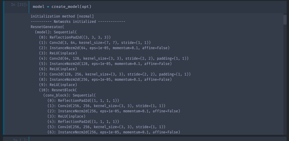
We've got our model and remember the model contains the loss functions, generators, discriminators, all in one convenient place [2:09:32]. I've gone ahead and copied and pasted and slightly refactored the training loop from their code so that we can run it inside the notebook. So this one should look a lot familiar. A loop to go through each epoch and a loop to go through the data. Before we did this, we set up dataset. This is actually not a PyTorch dataset, I think this is what they used slightly confusingly to talk about their combined what we would call a model data object — all the data that they need. Loop through that with tqdm to get a progress bar, and so now we can go through and see what happens in the model.

# note: Jeremy's refactor also removed all the visualizer codes

def train(total_steps=0):
    for epoch in range(opt.epoch_count, opt.niter + opt.niter_decay + 1):
        epoch_start_time = time.time()
        iter_data_time = time.time()
        epoch_iter = 0

        for i, data in tqdm(enumerate(dataset)):
            iter_start_time = time.time()
            if total_steps % opt.print_freq == 0: t_data = iter_start_time - iter_data_time
            total_steps += opt.batchSize
            epoch_iter += opt.batchSize
            model.set_input(data)
            model.optimize_parameters()

            if total_steps % opt.display_freq == 0:
                save_result = total_steps % opt.update_html_freq == 0

            if total_steps % opt.print_freq == 0:
                errors = model.get_current_errors()
                t = (time.time() - iter_start_time) / opt.batchSize

            if total_steps % opt.save_latest_freq == 0:
                print('saving the latest model (epoch %d, total_steps %d)' % (epoch, total_steps))
                model.save('latest')

            iter_data_time = time.time()
        if epoch % opt.save_epoch_freq == 0:
            print('saving the model at the end of epoch %d, iters %d' % (epoch, total_steps))
            model.save('latest')
            model.save(epoch)

        print('End of epoch %d / %d \t Time Taken: %d sec' %
              (epoch, opt.niter + opt.niter_decay, time.time() - epoch_start_time))
        model.update_learning_rate()

%time train(0)

set_input [2:10:32]: It's a different approach to what we do in fastai. This is kind of neat, it's quite specific to Cycle GANs but basically internally inside this model is this idea that we are going to go into our data and grab the appropriate one. We are either going horse to zebra or zebra to horse, depending on which way we go, A is either horse or zebra, and vice versa. If necessary put it on the appropriate GPU, then grab the appropriate paths. So the model now has a mini-batch of horses and a mini-batch of zebras.

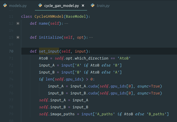
Now we optimize the parameters [2:11:19]. It's kind of nice to see it like this. You can see each step. First of all, try to optimize the generators, then try to optimize the horse discriminators, then try to optimize the zebra discriminator. zero_grad() is a part of PyTorch, as well as step(). So the interesting bit is the actual thing that does the back propagation on the generator.

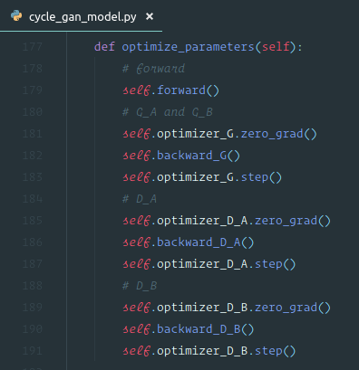
Here it is [2:12:04]. Let's jump to the key pieces. There's all the formula that we just saw in the paper. Let's take a horse and generate a zebra. Let's now use the discriminator to see if we can tell whether it's fake or not (pred_fake). Then let's pop that into our loss function which we set up earlier to get a GAN loss based on that prediction. Let's do the same thing going the opposite direction using the opposite discriminator then put that through the loss function again. Then let's do the cycle consistency loss. Again, we take our fake which we created and try and turn it back again into the original. Let's use the cycle consistency loss function we created earlier to compare it to the real original. And here is that lambda — so there's some weight that we used and that would set up, actually we just use the default that they suggested in their options. Then do the same for the opposite direction and then add them all together. We then do the backward step. That's it.

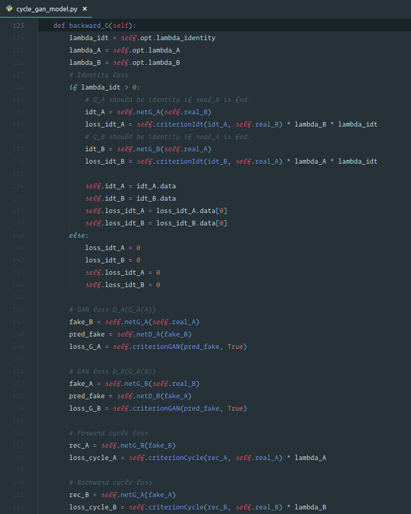
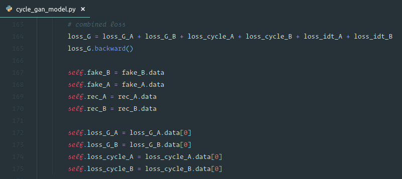
So we can do the same thing for the first discriminator [2:13:50]. Since basically all the work has been done now, there's much less to do here. There that is. We won't step all through it but it's basically the same basic stuff that we've already seen.

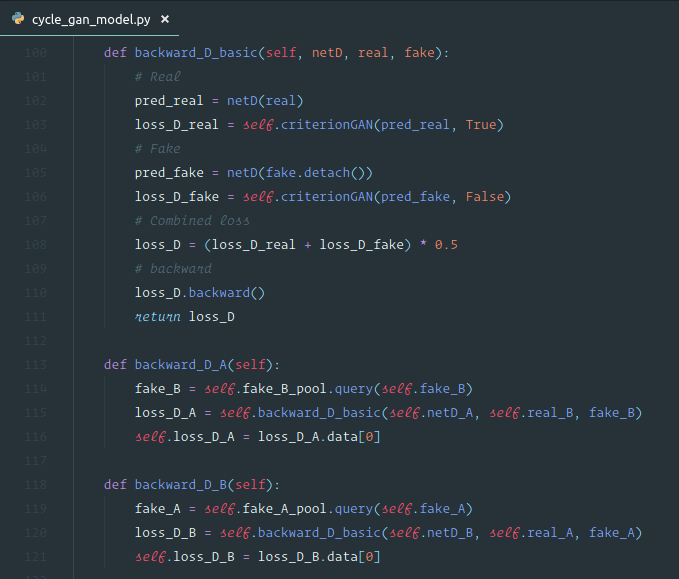
So optimize_parameters() is calculating the losses and doing the optimizer step. From time to time, save and print out some results. Then from time to time, update the learning rate so they've got some learning rate annealing built in here as well. Kind of like fast.ai, they've got this idea of schedulers which you can then use to update your learning rates.

For those of you are interested in better understanding deep learning APIs, contributing more to fast.ai, or creating your own version of some of this stuff in some different back-end, it's cool to look at a second API that covers some subset of some of the similar things to get a sense for how they are solving some of these problems and what the similarities/differences are.

def show_img(im, ax=None, figsize=None):
    if not ax: fig, ax = plt.subplots(figsize=figsize)
    ax.imshow(im)
    ax.get_xaxis().set_visible(False)
    ax.get_yaxis().set_visible(False)
    return ax

We train that for a little while and then we can just grab a few examples and here we have them [2:15:29]. Here are horses, zebras, and back again as horses.

After train for 4 epochs:

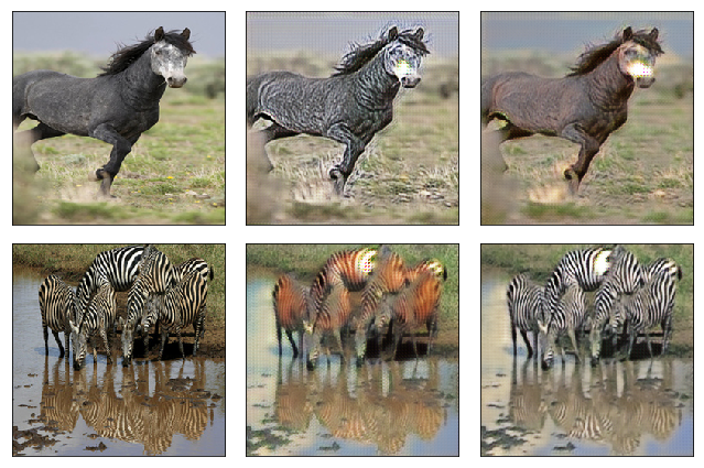
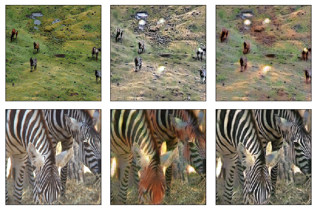
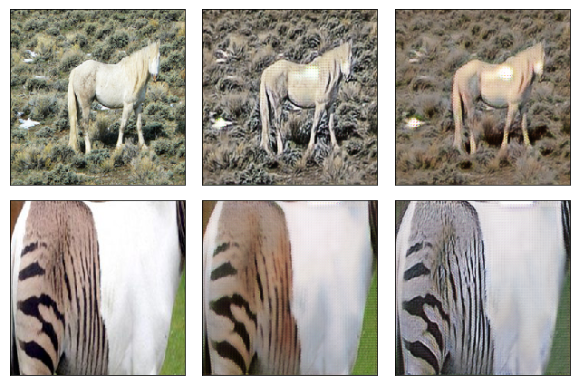
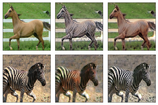
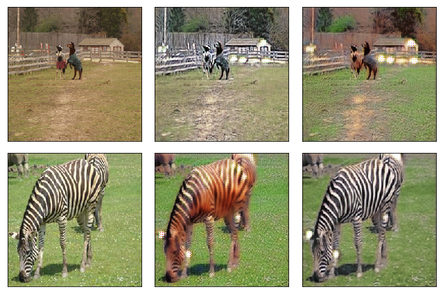
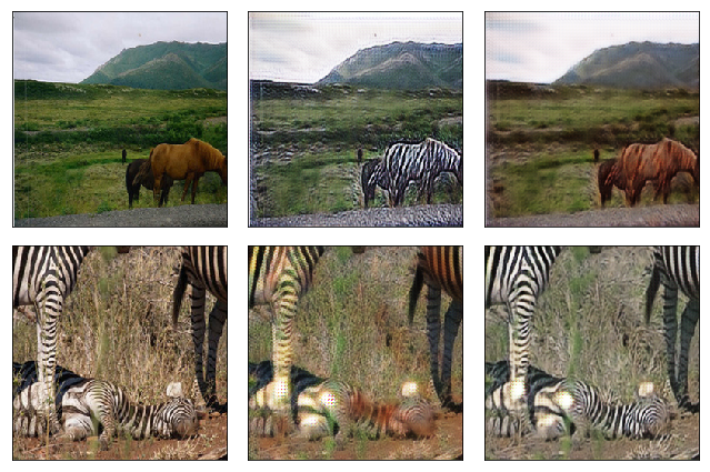
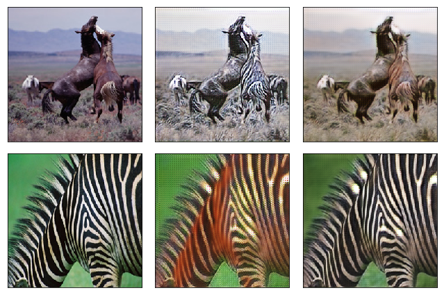
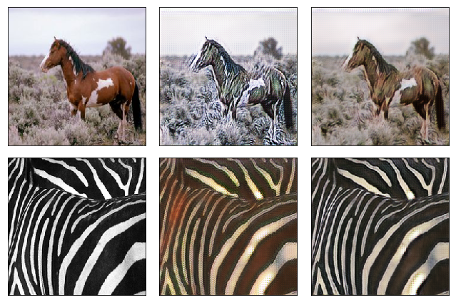
After train for 300 epochs + 100 epochs with learning rate annealing:

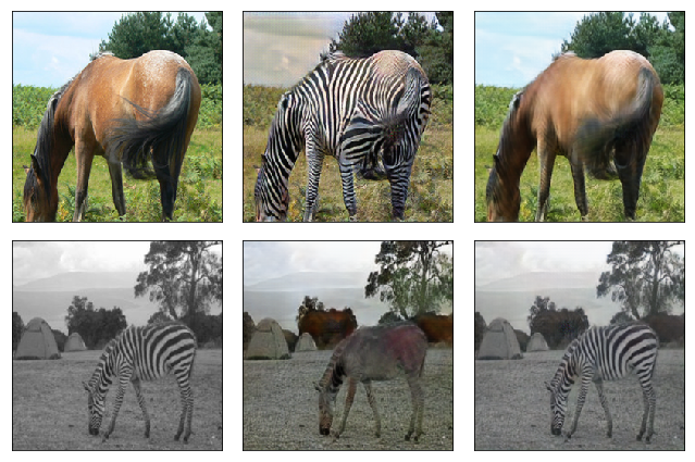
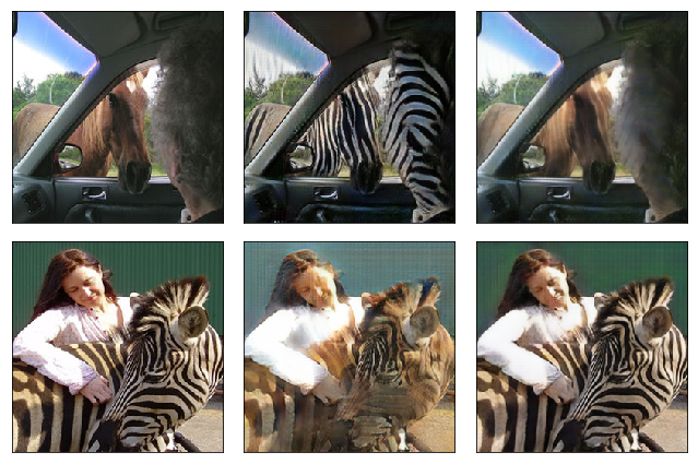
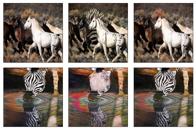
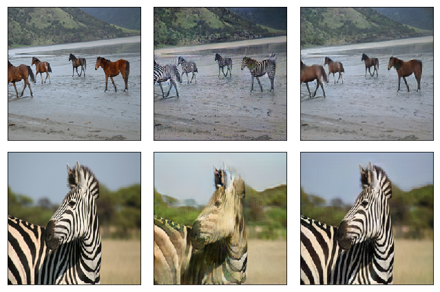
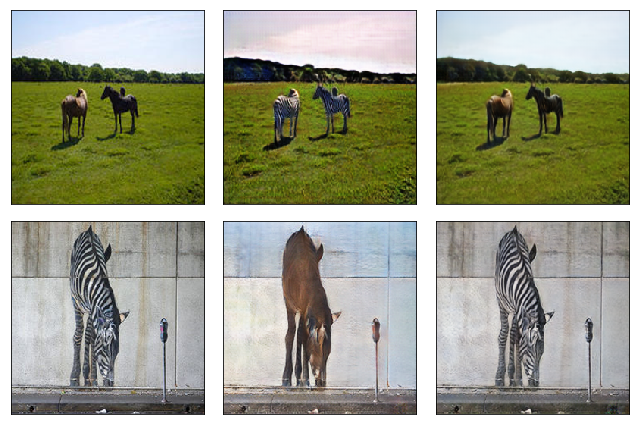
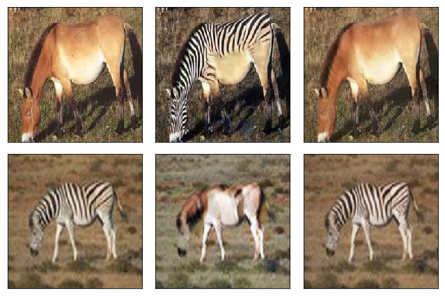
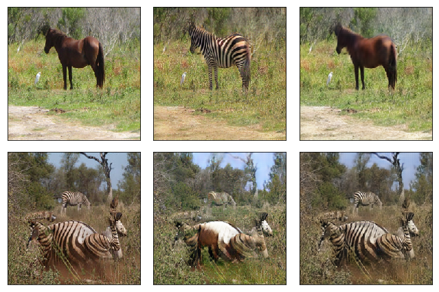
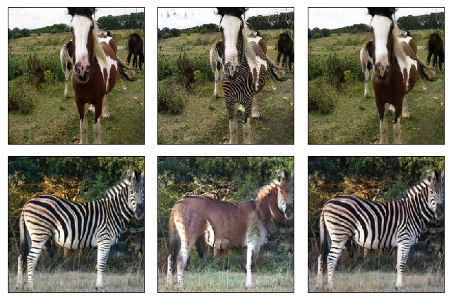
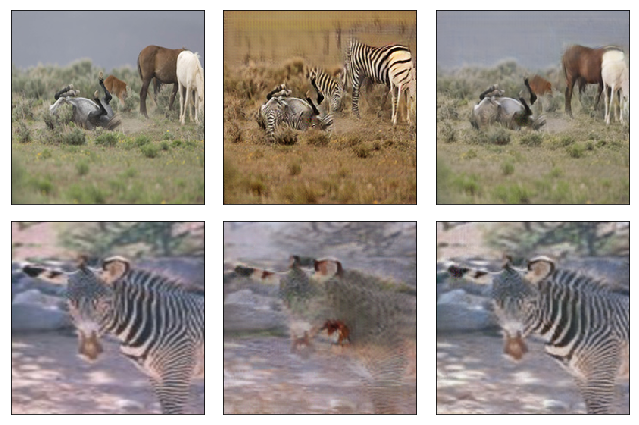
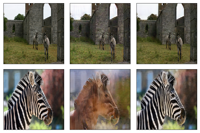
It took Jeremy like 24 hours to train it even that far so it's kind of slow [2:16:39]. I know Helena is constantly complaining on Twitter about how long these things take. I don't know how she's so productive with them.

🔖 note-to-self: try training on 8 GPUs and with a bigger batch size.

I will mention one more thing that just came out yesterday [2:16:54]:

Multimodal Unsupervised Image-to-Image Translation.

There is now a multi-modal image to image translation of unpaired. So you can basically now create different cats for instance from this dog.

This is basically not just creating one example of the output that you want, but creating multiple ones. This came out yesterday or the day before. I think it's pretty amazing. So you can kind of see how this technology is developing and I think there's so many opportunities to maybe do this with music, speech, writing, or to create kind of tools for artists.

Lesson 12 - DarkNet; Generative Adversarial Networks (GANs)

Topics​

Lesson Resources​

Assignments​

Papers​

Other Resources​

Other Useful Information​

My Notes​

Generative Adversarial Networks (GANs)​

CIFAR10 [00:05:26]​

cifar10-darknet.ipynb [00:07:17]​

Leaky ReLU [00:12:43]:​

Residual block [00:14:40]:​

Wide Residual Networks​

DAWNBench [00:37:43]​

Generative Adversarial Networks (GAN) [00:48:49]​

Looking at the code [00:54:52]​

Discriminator​

Generator [1:06:15]​

Deconvolution [1:09:36]​

ConvTranspose2d [1:16:00]​

Visualizing [1:16:33]​

Putting them all together [1:24:30]​

Cycle GAN [1:41:08]​

Cycle-consistency loss [1:57:14]​

Full objective [1:58:54]​

Implementing Cycle GAN [2:00:41]​