Lesson 11 - Neural Translation; Multi-modal Learning

These are my personal notes from fast.ai course and will continue to be updated and improved if I find anything useful and relevant while I continue to review the course to study much more in-depth. Thanks for reading and happy learning!

Topics

• Learn to translate French into English.
  • How to add attention to an LSTM in order to build a sequence to sequence (seq2seq) model.
  • Review of some key RNN foundations, since a solid understanding of those will be critical to understanding the rest of this lesson.
• A seq2seq model is one where both the input and the output are sequences, and can be of difference lengths.
• Learn an attention mechanism to figure out which words to focus on at each time step.
• Tricks to improve seq2seq results, including teacher forcing and bidirectional models.
• Discuss the DeViSE paper, which shows how we can bridge the divide between text and images, using them both in the same model.

Lesson Resources

• Website
• Video
• Wiki
• Jupyter Notebook and code
  • translate.ipynb
  • devise.ipynb
• Dataset
  • Parallel Giga French-English corpus / direct download link (2.3 GB)
  • ImageNet train set sample (a subset of the full ImageNet data which is a large 156 GB)

Assignments

Papers

• Must read
  • Google's Neural Machine Translation System: Bridging the Gap between Human and Machine Translation
  • Neural Machine Translation by Jointly Learning to Align and Translate by Dzmitry Bahdanau, Kyunghyun Cho, Yoshua Bengio - original paper explaining the attention approach explained in class
  • Grammar as a Foreign Language by Oriol Vinyals, Geoffrey Hinton, et. al - concise summary of attention in this paper
  • DeViSE: A Deep Visual-Semantic Embedding Model
• Additional papers (optional)
  • Papers and SoTA results
  • BLEU: a Method for Automatic Evaluation of Machine Translation - understanding BiLingual Evaluation Understudy (BLEU) score

Other Resources

Other Useful Information

• Stephen Merity's talk on Attention and Memory in Deep Learning Networks

Useful Tools and Libraries

• Tensor2Tensor - a Google DL mini-library with many datasets and tutorials for various seq2seq tasks

Code Snippets

• Useful function to transform PyTorch nn.module class to fastai Learner class

  rnn = Seq2SeqRNN(fr_vecd, fr_itos, dim_fr_vec, en_vecd, en_itos, dim_en_vec, nh, enlen_90)
  learn = RNN_Learner(md, SingleModel(to_gpu(rnn)), opt_fn=opt_fn)

My Notes

Before getting started:

• The 1cycle policy by Sylvain Gugger. Based on Leslie Smith's new paper which takes the previous two key papers (cyclical learning rate and super convergence) and built on them with a number of experiments to show how you can achieve super convergence. Super convergence lets you train models five times faster than the previous stepwise approach (and faster than CLR, although it is less than five times). Super convergence lets you get up to massively high learning rates by somewhere between 1 and 3. The interesting thing about super convergence is that you train at those very high learning rates for quite a large percentage of your epochs and during that time, the loss doesn't really improve very much. But the trick is it's doing a lot of searching through the space to find really generalizable areas it seems. Sylvain implemented it in fastai by flushing out the pieces that were missing then confirmed that he actually achieved super convergence on training on CIFAR10. It is currently called use_clr_beta but will be renamed in future. He also added cyclical momentum to fastai library.
• How To Create Data Products That Are Magical Using Sequence-to-Sequence Models by Hamel Husain. He blogged about training a model to summarize GitHub issues. Here is the demo Kubeflow team created based on his blog.

Neural Machine Translation [00:05:36]

Let's build a sequence-to-sequence model! We are going to be working on machine translation. Machine translation is something that's been around for a long time, but we are going to look at an approach called neural translation which uses neural networks for translation. Neural machine translation appeared a couple years ago and it was not as good as the statistical machine translation approaches that use classic feature engineering and standard NLP approaches like stemming, fiddling around with word frequencies, n-grams, etc. By a year later, it was better than everything else. It is based on a metric called BLEU — we are not going to discuss the metric because it is not a very good metric and it is not interesting, but everybody uses it.

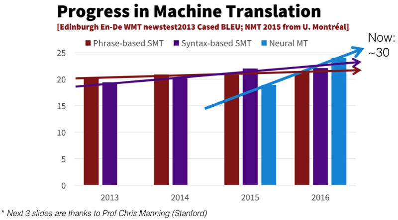
We are seeing machine translation starting down the path that we saw starting computer vision object classification in 2012 which just surpassed the state-of-the-art and now zipping past it at great rate. It is unlikely that anybody watching this is actually going to build a machine translation model because https://translate.google.com/ works quite well. So why are we learning about machine translation? The reason we are learning about machine translation is that the general idea of taking some kind of input like a sentence in French and transforming it into some other kind of output with arbitrary length such as a sentence in English is a really useful thing to do. For example, as we just saw, Hamel took GitHub issues and turn them into summaries. Another example is taking videos and turning them into descriptions, or basically anything where you are spitting out an arbitrary sized output which is very often a sentence. Maybe taking a CT scan and spitting out a radiology report — this is where you can use sequence to sequence learning.

Four big wins of Neural Machine Translation [00:08:36]

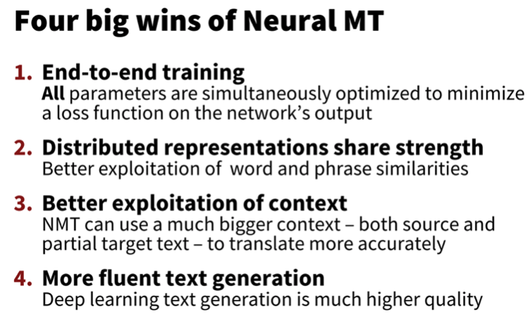
• End-to-end training: No fussing around with heuristics and hacky feature engineering.
• We are able to build these distributed representations which are shared by lots of concepts within a single network.
• We are able to use long term state in the RNN so it uses a lot more context than n-gram type approaches.
• In the end, text we are generating uses RNN as well so we can build something that is more fluid.

BiLSTMs(+Attention) not just for neural MT [00:09:20]

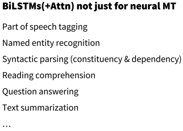
We are going to use bi-directional GRU (basically the same as LSTM) with attention — these general ideas can also be used for lots of other things as you see above.

Let's jump into the code [00:09:47]

translate.ipynb

We are going to try to translate French into English by following the standard neural network approach:

1. Data
2. Architecture
3. Loss Function

1. Data

As usual, we need (x, y) pair. In this case, x: French sentence, y: English sentence which you will compare your prediction against. We need lots of these tuples of French sentences with their equivalent English sentence — that is called "parallel corpus" and harder to find than a corpus for a language model. For a language model, we just need text in some language. For any living language, there will be a few gigabytes at least of text floating around the Internet for you to grab. For translation, there are some pretty good parallel corpus available for European languages. The European Parliament has every sentence in every European language. Anything that goes to the UN is translated to lots of languages. For French to English, we have particularly nice thing which is pretty much any semi official Canadian website will have a French version and an English version[00:12:13].

Translation files

from fastai.text import *

French-English parallel texts from http://www.statmt.org/wmt15/translation-task.html . It was created by Chris Callison-Burch, who crawled millions of web pages and then used a set of simple heuristics to transform French URLs onto English URLs (i.e. replacing "fr" with "en" and about 40 other hand-written rules), and assume that these documents are translations of each other.

PATH = Path('data/translate')
TMP_PATH = PATH / 'tmp'
TMP_PATH.mkdir(exist_ok=True)
fname = 'giga-fren.release2.fixed'
en_fname = PATH / f'{fname}.en'
fr_fname = PATH / f'{fname}.fr'

For bounding boxes, all of the interesting stuff was in the loss function, but for neural translation, all of the interesting stuff is going to be in the architecture [00:13:01]. Let's zip through this pretty quickly and one of the things Jeremy wants you to think about particularly is what are the relationships or the similarities in terms of the tasks we are doing and how we do it between language modeling vs. neural translation.

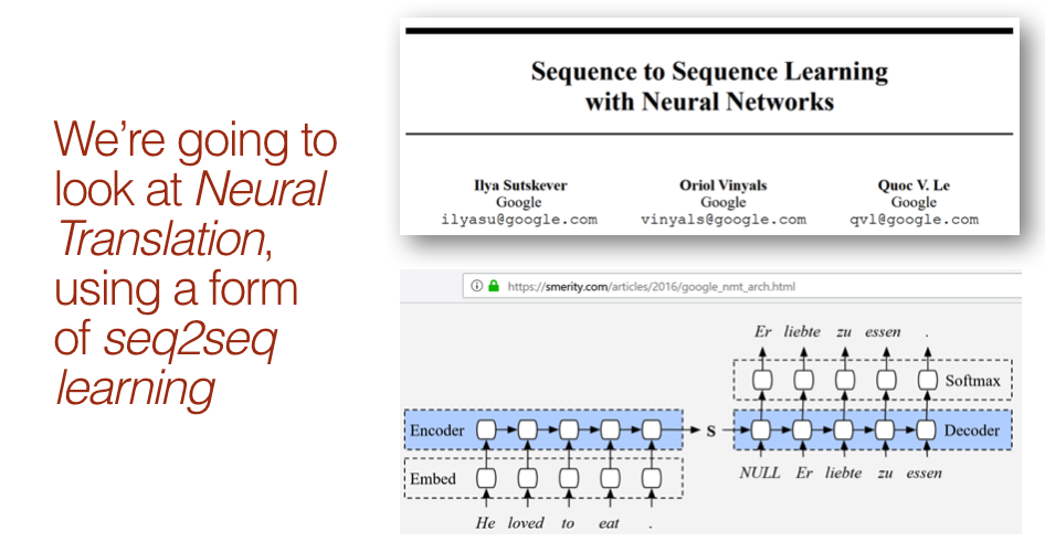
The first step is to do the exact same thing we do in a language model which is to take a sentence and chuck it through an RNN[00:13:35].

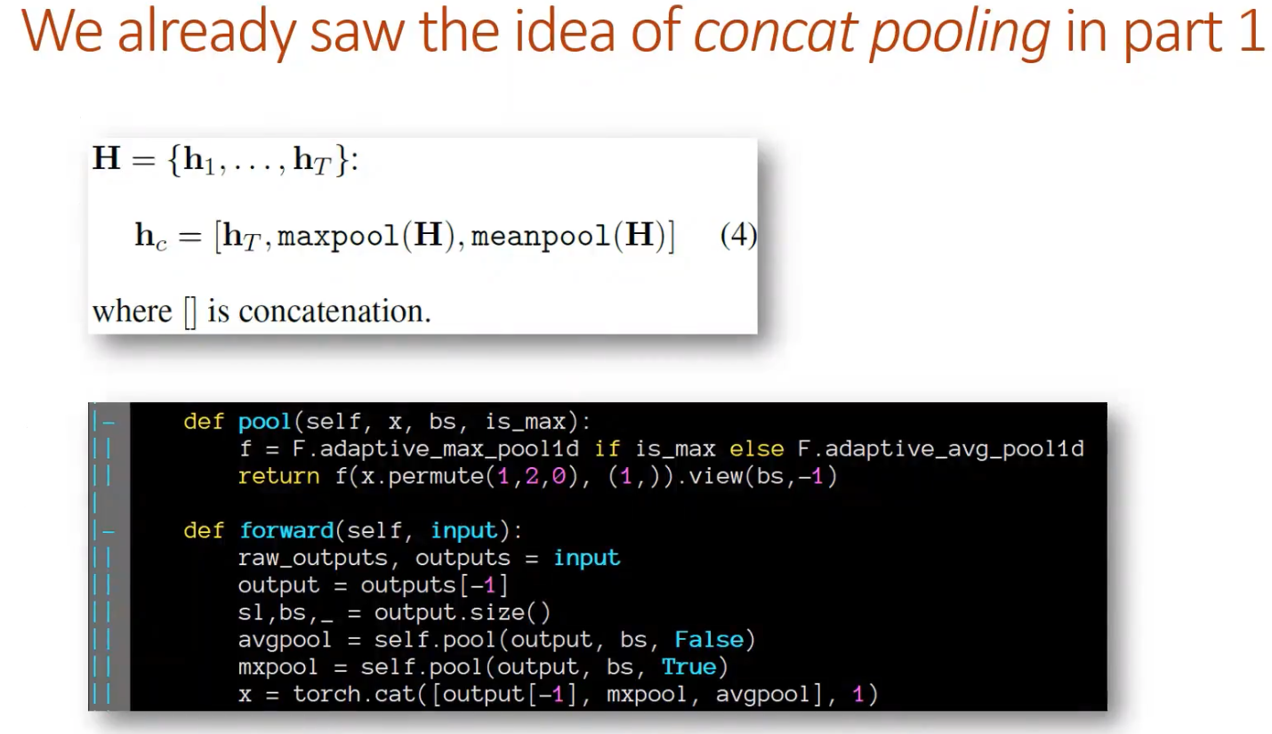
Now with the classification model, we had a decoder which took the RNN output and grabbed three things: maxpool and meanpool over all of the time steps, and the value of the RNN at the last time step, stack all those together and put it through a linear layer [00:14:24]. Most people do not do that and just use the last time step, so all the things we will be talking about today uses the last time step.

We start out by chucking the input sentence through an RNN and out of it comes some "hidden state" (i.e. some vector that represents the output of an RNN that has encoded the sentence).

Encoder ≈ Backbone [00:15:18]

Stephen used the word "encoder", but we tend to use the word "backbone". Like when we talked about adding a custom head to an existing model, the existing pre-trained ImageNet model, for example, we say that is our backbone and then we stick on top of it some head that does the task we want. In sequence to sequence learning, they use the word encoder, but it basically is the same thing — it is some piece of a neural network architecture that takes the input and turns it into some representation which we can then stick a few more layers on top to grab something out of it such as we did for the classifier where we stack a linear layer on top of it to turn int into a sentiment. This time though, we have something that's a little bit harder than just creating sentiment [00:16:12]. Instead of turning the hidden state into a positive or negative sentiment, we want to turn it into a sequence of tokens where that sequence of token is the German sentence in Stephen's example.

This is sounding more like the language model than the classifier because the language had multiple tokens (for every input word, there was an output word). But the language model was also much easier because the number of tokens in the language model output was the same length as the number of tokens in the language model input. Not only they were the same length, but they exactly matched up (e.g. after word one comes word two, after word two comes word three, and so forth). For translating language, you don't necessarily know that the word "he" will be translated as the first word in the output (unfortunately, it is in this particular case). Very often, the subject object order will be different or there will be some extra words inserted, or some pronouns we will need to add some gendered article, etc. This is the key issue we are going to have to deal with is the fact that we have an arbitrary length output where the tokens in the output do not correspond to the same order or the specific tokens in the input [00:17:31]. But the general idea is the same. Here is an RNN to encode the input, turns it into some hidden state, then this is the new thing we are going to learn is generating a sequence output.

Sequence output [00:17:47]

We already know:

• Sequence to class (IMDB classifier)
• Sequence to equal length sequence (Language model)

But we do not know yet how to do a general purpose sequence to sequence, so that's the new thing today. Very little of this will make sense unless you really understand lesson 6 how an RNN works.

Quick review of Lesson 6 [00:18:20]

We learnt that an RNN at its heart is a standard fully connected network. Below is one with 4 layers — takes an input and puts it through four layers, but at the second layer, it concatenates in the second input, third layer concatenated in the third input, but we actually wrote this in Python as just a four layer neural network. There was nothing else we used other than linear layers and ReLUs. We used the same weight matrix every time when an input came in, we used the same matrix every time when we went from one of the hidden states to the next — that is why these arrows are the same color.

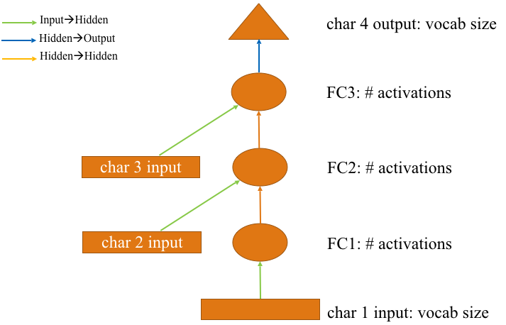
We can redraw the above diagram like the below [00:19:29].

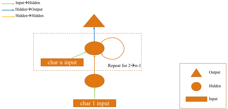
Not only did we redraw it but we took the four lines of linear code in PyTorch and we replaced it with a for loop. Remember, we had something that did exactly the same thing as below, but it just had four lines of code saying self.l_in(input) and we replaced it with a for loop because that's nice to refactor. The refactoring which does not change any of the math, any of the ideas, or any of the outputs is an RNN. It's turning a bunch of separate lines in the code into a Python for loop.

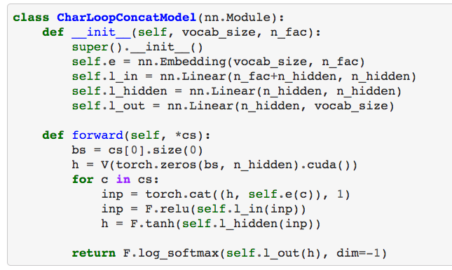
We could take the output so that it is not outside the loop and put it inside the loop [00:20:25]. If we do that, we are now going to generate a separate output for every input. The code above, the hidden state gets replaced each time and we end up just spitting out the final hidden state. But if instead, we had something that said hs.append(h) and returned hs at the end, that would be the picture below.

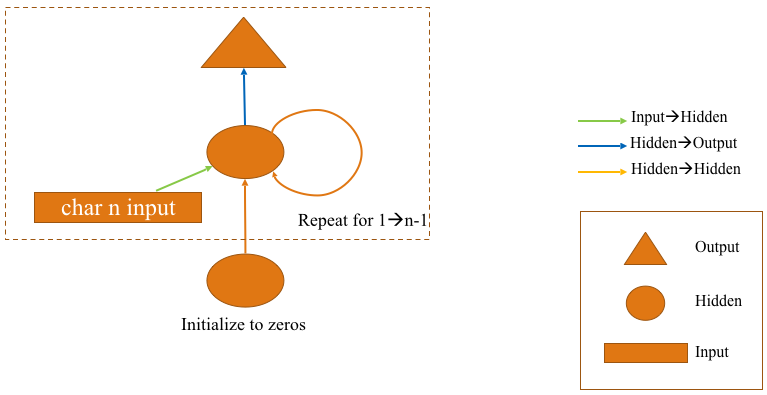
The main thing to remember is when we say hidden state, we are referring to a vector — technically a vector for each thing in the mini-batch so it's a matrix, but generally when Jeremy speaks about these things, he ignores the mini-batch piece and treat it for just a single item.

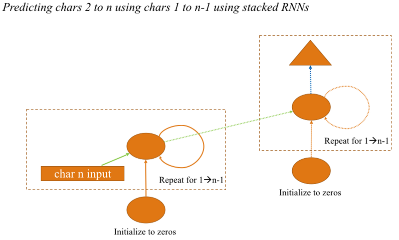
We also learned that you can stack these layers on top of each other [00:21:41]. So rather than the left RNN (in the diagram above) spitting out output, they could just spit out inputs into a second RNN. If you are thinking at this point "I think I understand this but I am not quite sure" that means you don't understand this. The only way you know that you actually understand it is to go and write this from scratch in PyTorch or Numpy. If you can't do that, then you know you don't understand it and you can go back and re-watch lesson 6 and check out the notebook and copy some of the ideas until you can. It is really important that you can write that from scratch — it's less than a screen of code. So you want to make sure you can create a 2 layer RNN. Below is what it looks like if you unroll it.

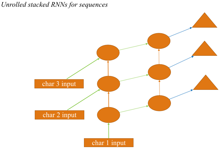
To get to a point that we have (x, y) pairs of sentences, we will start by downloading the dataset [00:22:39]. Training a translation model takes a long time. Google's translation model has eight layers of RNN stacked on top of each other. There is no conceptual difference between eight layers and two layers. If you are Google and you have more GPUs or TPUs than you know what to do with, then you are fine doing that. Where else, in our case, it's pretty likely that the kind of sequence to sequence models we are building are not going to require that level of computation. So to keep things simple [00:23:22], let's do a cut-down thing where rather than learning how to translate French into English for any sentence, let's learn to translate French questions into English questions — specifically questions that start with what/where/which/when. So here is a regex which looks for things that start with "wh" and end with a question mark.

# Question regex search filters
re_eq = re.compile('^(Wh[^?.!]+\?)')
re_fq = re.compile('^([^?.!]+\?)')

# grabbing lines from the English and French source texts
lines = ( (re_eq.search(eq), re_fq.search(fq))
         for eq, fq in zip(open(en_fname, encoding='utf-8'), open(fr_fname, encoding='utf-8')))

# isolate the questions
qs = [(e.group(), f.group()) for e, f in lines if e and f]

We go through the corpus [00:23:43], open up each of the two files, each line is one parallel text, zip them together, grab the English question and the French question, and check whether they match the regular expressions.

# save the questions for later
pickle.dump(qs, (PATH / 'fr-en-qs.pkl').open('wb'))

# load in pickled questions
qs = pickle.load((PATH / 'fr-en-qs.pkl').open('rb'))

Dump that out as a pickle so we don't have to do it again and so now we have 52,000 sentence pairs and here are some examples:

print(len(qs))
print(qs[:5])

# -----------------------------------------------------------------------------
# Output
# -----------------------------------------------------------------------------
52331
[('What is light ?', 'Qu'est-ce que la lumière?'), ('Who are we?', 'Où sommes-nous?'), ('Where did we come from?', "D'où venons-nous?"), ('What would we do without it?', 'Que ferions-nous sans elle ?'), ('What is the absolute location (latitude and longitude) of Badger, Newfoundland and Labrador?', 'Quelle sont les coordonnées (latitude et longitude) de Badger, à Terre-Neuve-etLabrador?')]

One nice thing about this is that what/who/where type questions tend to be fairly short [00:24:08]. But the idea that we could learn from scratch with no previous understanding of the idea of language let alone of English or French that we could create something that can translate one to the other for any arbitrary question with only 50k sentences sounds like a ludicrously difficult thing to ask this to do. So it would be impressive if we can make any progress what so ever. This is very little data to do a very complex exercise.

qs contains the tuples of French and English [00:24:48]. You can use this handy idiom to split them apart into a list of English questions and a list of French questions.

en_qs, fr_qs = zip(*qs)

Then we tokenize the English questions and tokenize the French questions. So remember that just means splitting them up into separate words or word-like things. By default [00:25:11], the tokenizer that we have here (remember this is a wrapper around the spaCy tokenizer which is a fantastic tokenizer) assumes English. So to ask for French, you just add an extra parameter 'fr'. The first time you do this, you will get an error saying you don't have the spaCy French model installed so you can run python -m spacy download fr to grab the French model.

en_tok = Tokenizer.proc_all_mp(partition_by_cores(en_qs))
fr_tok = Tokenizer.proc_all_mp(partition_by_cores(fr_qs), 'fr')

It is unlikely that any of you are going to have RAM problems here because this is not particularly big corpus but some of the students were trying to train a new language models during the week and were having RAM problems. If you do, it's worth knowing what these functions (proc_all_mp) are actually doing. proc_all_mp is processing every sentence across multiple processes [00:25:59]:

The function above finds out how many CPUs you have, divide it by two (because normally with hyper-threading they don't actually all work in parallel), then in parallel run this proc_all function. So that is going to spit out a whole separate Python processes for every CPU you have. If you have a lot of cores, that is a lot of Python processes — everyone is going to load all this data in and that can potentially use up all your RAM. So you could replace that with just proc_all rather than proc_all_mp to use less RAM. Or you could just use less cores. At the moment, we are calling partition_by_cores which calls partition on a list and asks to split it into a number of equal length things according to how many CPUs you have. So you could replace that to split into a smaller list and run it on less things.

Having tokenized the English and French, you can see how it gets split up [00:28:04]:

en_tok[:3], fr_tok[:3]

# -----------------------------------------------------------------------------
# Output
# -----------------------------------------------------------------------------
([['what', 'is', 'light', '?'],
  ['who', 'are', 'we', '?'],
  ['where', 'did', 'we', 'come', 'from', '?']],
 [['qu'', 'est', '-ce', 'que', 'la', 'lumière', '?'],
  ['où', 'sommes', '-', 'nous', '?'],
  ["d'", 'où', 'venons', '-', 'nous', '?']])

You can see the tokenization for French is quite different looking because French loves their apostrophes and their hyphens. So if you try to use an English tokenizer for a French sentence, you're going to get a pretty crappy outcome. You don't need to know heaps of NLP ideas to use deep learning for NLP, but just some basic stuff like use the right tokenizer for your language is important [00:28:23]. Some of the students this week in our study group have been trying to build language models for Chinese instance which of course doesn't really have the concept of a tokenizer in the same way, so we've been starting to look at SentencePiece which splits things into arbitrary sub-word units and so when Jeremy says tokenize, if you are using a language that doesn't have spaces in, you should probably be checking out SentencePiece or some other similar sub-word unit thing instead. Hopefully in the next week or two, we will be able to report back with some early results of these experiments with Chinese.

# 90th percentile of English and French sentences length.
np.percentile([len(o) for o in en_tok], 90), np.percentile([len(o) for o in fr_tok], 90)

# -----------------------------------------------------------------------------
# Output
# -----------------------------------------------------------------------------
(23.0, 28.0)

# We are keeping tokens that are less than 30 chars. The filter is applied on the English words, and the same tokens are kept for French.
keep = np.array([len(o) < 30 for o in en_tok])

en_tok = np.array(en_tok)[keep]
fr_tok = np.array(fr_tok)[keep]

# save our work
pickle.dump(en_tok, (PATH / 'en_tok.pkl').open('wb'))
pickle.dump(fr_tok, (PATH / 'fr_tok.pkl').open('wb'))

en_tok = pickle.load((PATH / 'en_tok.pkl').open('rb'))
fr_tok = pickle.load((PATH / 'fr_tok.pkl').open('rb'))

So having tokenized it [00:29:25], we will save that to disk. Then remember, the next step after we create tokens is to turn them into numbers. To do that, we have two steps — the first is to get a list of all of the words that appear and then we turn every word into the index. If there are more than 40,000 words that appear, then let's cut it off there so it doesn't go too crazy. We insert a few extra tokens for beginning of stream (_bos_), padding (_pad_), end of stream (_eos_), and unknown (_unk). So if we try to look up something that wasn't in the 40,000 most common, then we use a defaultdict to return 3 which is unknown.

def toks2ids(tok, pre):
    """
    Numericalize words to integers.

    Arguments:
        tok: token
        pre: prefix
    """
    freq = Counter(p for o in tok for p in o)
    itos = [o for o, c in freq.most_common(40000)] # 40k most common words
    itos.insert(0, '_bos_')
    itos.insert(1, '_pad_')
    itos.insert(2, '_eos_')
    itos.insert(3, '_unk')
    stoi = collections.defaultdict(lambda: 3, { v: k for k, v in enumerate(itos) }) #reverse
    ids = np.array([ ([stoi[o] for o in p] + [2]) for p in tok ])
    np.save(TMP_PATH / f'{pre}_ids.npy', ids)
    pickle.dump(itos, open(TMP_PATH / f'{pre}_itos.pkl', 'wb'))
    return ids, itos, stoi

Now we can go ahead and turn every token into an ID by putting it through the string to integer dictionary (stoi) we just created and then at the end of that let's add the number 2 which is the end of stream. The code you see here is the code Jeremy writes when he is iterating and experimenting [00:30:25]. Because 99% of the code he writes while iterating and experimenting turns out to be totally wrong or stupid or embarrassing and you don't get to see it. But there is not point refactoring that and making it beautiful when he's writing it so he wanted you to see all the little shortcuts he has. Rather than having some constant for _eos_ marker and using that, when he is prototyping he just does the easy stuff. Not so much that he ends up with broken code but he tries to find some middle ground between beautiful code and code that works.

❓ Just heard him mention that we divide the number of CPUs by 2 because with hyper-threading, we don't get a speed-up using all the hyper threaded cores. Is this based on practical experience or is there some underlying reason why we wouldn't get additional speedup [00:31:18]?

Yes, it's just practical experience and it's not all things seemed like this, but I definitely noticed with tokenization — hyper-threading seemed to slow things down a little bit. Also if I use all the cores, often I want to do something else at the same time (like running some interactive notebook) and I don't have any spare room to do that.

Now for our English and French, we can grab a list of IDs en_ids [00:32:01]. When we do that, of course, we need to make sure that we also store the vocabulary. There is no point having IDs if we don't know what a number 5 represents, there is no point having a number 5. So that's our vocabulary en_itos and reverse mapping en_stoi that we can use to convert more corpuses in the future.

en_ids, en_itos, en_stoi = toks2ids(en_tok, 'en')
fr_ids, fr_itos, fr_stoi = toks2ids(fr_tok, 'fr')

Just to confirm it's working, we can go through each ID, convert the int to a string, and spit that out — there we have our sentence back now with an end of stream marker at the end. Our English vocab is 17,000 and our French vocab is 25,000, so that's not too big and not too complex vocab that we are dealing with.

def load_ids(pre):
    ids = np.load(TMP_PATH / f'{pre}_ids.npy')
    itos = pickle.load(open(TMP_PATH / f'{pre}_itos.pkl', 'rb'))
    stoi = collections.defaultdict(lambda: 3, { v: k for k, v in enumerate(itos) })
    return ids, itos, stoi

en_ids, en_itos, en_stoi = load_ids('en')
fr_ids, fr_itos, fr_stoi = load_ids('fr')

# Sanity check
[fr_itos[o] for o in fr_ids[0]], len(en_itos), len(fr_itos)

# -----------------------------------------------------------------------------
# Output
# -----------------------------------------------------------------------------
(['qu'', 'est', '-ce', 'que', 'la', 'lumière', '?', '_eos_'], 17573, 24793)

Word vectors [00:32:53]

We spent a lot of time on the forum during the week discussing how pointless word vectors are and how you should stop getting so excited about them — and now we are going to use them. Why? All the stuff we've been learning about using language models and pre-trained proper models rather than pre-trained linear single layers which is what word vectors are, applies equally well to sequence to sequence. But Jeremy and Sebastian are starting to look at that. There is a whole thing for anybody interested in creating some genuinely new highly publishable results, the entire area of sequence to sequence with pre-trained language models has not been touched yet. Jeremy believes it is going to be just as good as classifications. If you work on this and you get to the point where you have something that is looking exciting and you want help publishing it, Jeremy is very happy to help co-author papers. So feel free to reach out when you have some interesting results.

At this stage, we do not have any of that, so we are going to use very little fastai [00:34:14]. All we have is word vectors — so let's at least use decent word vectors. Word2vec is very old word word vectors. There are better word vectors now and fastText is a pretty good source of word vectors. There is hundreds of languages available for them, and your language is likely to be represented.

fastText word vectors available from https://fasttext.cc/docs/en/english-vectors.html

fasttext Python library is not available in PyPI but here is a handy trick [00:35:03]. If there is a GitHub repo that has a setup.py and requirements.txt in it, you can just chuck git+ at the start then stick that in your pip install and it works. Hardly anybody seems to know this and if you go to the fastText repo, they won't tell you this — they'll say you have to download it and cd into it and blah but you don't. You can just run this:

!pip install git+https://github.com/facebookresearch/fastText.git

Download word vectors:

To use the fastText library, you'll need to download fastText word vectors for your language (download the ‘bin plus text' ones).

We are using the pre-trained word vectors for English and French language, trained on Wikipedia using fastText. These vectors in dimension 300 were obtained using the skip-gram model.

!aria2c --file-allocation=none -c -x 5 -s 5 -d data/translate https://s3-us-west-1.amazonaws.com/fasttext-vectors/wiki.en.zip

!aria2c --file-allocation=none -c -x 5 -s 5 -d data/translate https://s3-us-west-1.amazonaws.com/fasttext-vectors/wiki.fr.zip

import fastText as ft

# use the fastText library
en_vecs = ft.load_model(str((PATH / 'wiki.en.bin')))
fr_vecs = ft.load_model(str((PATH / 'wiki.fr.bin')))

Above are our English and French models. There are a text version and a binary version. The binary version is faster, so we will use that. The text version is also a bit buggy. We are going to convert it into a standard Python dictionary to make it a bit easier to work with [00:35:55]. This is just going through each word with a dictionary comprehension and save it as a pickle dictionary:

def get_vecs(lang, ft_vecs):
    """
    Convert fastText word vectors into a standard Python dictionary to make it a bit easier to work with.
    This is just going through each word with a dictionary comprehension and save it as a pickle dictionary.

    get_word_vector:
        [method] get the vector representation of word.
    get_words:
        [method] get the entire list of words of the dictionary optionally
        including the frequency of the individual words. This
        does not include any subwords.
    """
    vecd = { w: ft_vecs.get_word_vector(w) for w in ft_vecs.get_words() }
    pickle.dump(vecd, open(PATH / f'wiki.{lang}.pkl', 'wb'))
    return vecd

en_vecd = get_vecs('en', en_vecs)
fr_vecd = get_vecs('fr', fr_vecs)

en_vecd = pickle.load(open(PATH / 'wiki.en.pkl', 'rb'))
fr_vecd = pickle.load(open(PATH / 'wiki.fr.pkl', 'rb'))

# Test
ft_vecs = en_vecs
ft_words = ft_vecs.get_words(include_freq=True)
ft_word_dict = { k: v for k, v in zip(*ft_words) }
ft_words = sorted(ft_word_dict.keys(), key=lambda x: ft_word_dict[x])
len(ft_words)

# -----------------------------------------------------------------------------
# Output
# -----------------------------------------------------------------------------
2519370

Now we have our pickle dictionary, we can go ahead and look up a word, for example, a comma [00:36:07]. That will return a vector. The length of the vector is the dimensionality of this set of word vectors. In this case, we have 300 dimensional English and French word vectors.

dim_en_vec = len(en_vecd[','])
dim_fr_vec = len(fr_vecd[','])
dim_en_vec, dim_fr_vec

# -----------------------------------------------------------------------------
# Output
# -----------------------------------------------------------------------------
(300, 300)

For reasons you will see in a moment, we also want to find out what the mean and standard deviation of our vectors are. So the mean is about zero and standard deviation is about 0.3.

# en_vecd type is dict
en_vecs = np.stack(list(en_vecd.values())) # convert dict_values to list and then stack it
en_vecs.mean(), en_vecs.std()

# -----------------------------------------------------------------------------
# Output
# -----------------------------------------------------------------------------
(0.0075652334, 0.29283327)

Model data [00:36:48]

Often corpuses have a pretty long tailed distribution of sequence length and it's the longest sequences that tend to overwhelm how long things take, how much memory is used, etc. So in this case, we are going to grab 99th to 97th percentile of the English and French and truncate them to that amount. Originally Jeremy was using 90 percentiles (hence the variable name):

enlen_90 = int(np.percentile([len(o) for o in en_ids], 99))
frlen_90 = int(np.percentile([len(o) for o in fr_ids], 99))
enlen_90, frlen_90

# -----------------------------------------------------------------------------
# Output
# -----------------------------------------------------------------------------
(29, 38)

Create our Dataset, DataLoaders

We are nearly there [00:37:24]. We've got our tokenized, numericalized English and French dataset. We've got some word vectors. So now we need to get it ready for PyTorch. PyTorch expects a Dataset object and hopefully by now you can say that a Dataset object requires two things — a length (__len__)and an indexer (__getitem__). Jeremy started out writing Seq2SeqDataset which turned out to be just a generic Dataset [00:37:52].

en_ids_tr = np.array([o[:enlen_90] for o in en_ids])
fr_ids_tr = np.array([o[:frlen_90] for o in fr_ids])

class Seq2SeqDataset(Dataset):
    def __init__(self, x, y):
        self.x, self.y = x, y

    def __getitem__(self, idx):
        return A(self.x[idx], self.y[idx]) # A for Arrays

    def __len__(self):
        return len(self.x)

• A : Arrays. It will go through each of the thing you pass it, if it is not already a numpy array, it converts into a numpy array and returns back a tuple of all of the things you passed it which are now guaranteed to be numpy arrays [00:38:32].
• V : Variables
• T : Tensors

Training set and validation set [00:39:03]

Now we need to grab our English and French IDs and get a training set and a validation set.

⚠️ One of the things which is pretty disappointing about a lot of code out there on the Internet is that they don't follow some simple best practices.

For example, if you go to PyTorch website, they have an example section for sequence to sequence translation. Their example does not have a separate validation set. Jeremy tried training according to their settings and tested it with a validation set and it turned out that it overfit massively. So this is not just a theoretical problem — the actual PyTorch repo has the actual official sequence to sequence translation example which does not check for overfitting and overfits horribly [00:39:41]. Also it fails to use mini-batches so it actually fails to utilize any of the efficiency of PyTorch whatsoever. Even if you find code in the official PyTorch repo, don't assume it's any good at all. The other thing you'll notice is that pretty much every other sequence to sequence model Jeremy found in PyTorch anywhere on the Internet has clearly copied from that crappy PyTorch repo because all has the same variable names, it has the same problems, it has the same mistakes.

Another example is that nearly every PyTorch convolutional neural network Jeremy found does not use an adaptive pooling layer [00:40:27]. So in other words, the final layer is always average pool (7, 7). They assume that the previous layer is 7 by 7 and if you use any other size input, you get an exception, and therefore nearly everybody Jeremy has spoken who uses PyTorch thinks that there is a fundamental limitation of CNNs that they are tied to the input size and that has not been true since VGG. So every time Jeremy grabs a new model and stick it in the fastai repo, he has to go and search for "pool" and add "adaptive" to the start and replace the 7 with a 1 and now it works on any sized object. So just be careful. It's still early days and believe it or not, even though most of you have only started in the last year your deep learning journey, you know quite a lot more about a lot of the more important practical aspects than the vast majority of people that have publishing and writing stuff in official repos. So you need to have a little more self-confidence than you might expect when it comes to reading other people's code. If you find yourself thinking "that looks odd", it's not necessarily you.

If the repo you are looking at doesn't have a section on it saying here is the test we did where we got the same results as the paper that's supposed to be implementing, that almost certainly means they haven't got the same results of the paper they're implementing, but probably haven't even checked [00:42:13]. If you run it, definitely won't get those results because it's hard to get things right the first time — it takes Jeremy 12 goes. If they haven't tested it once, it's almost certainly won't work.

Here is an easy way to get training and validation sets [00:42:45]. Grab a bunch of random numbers — one for each row of your data, and see if they are bigger than 0.1 or not. That gets you a list of booleans. Index into your array with that list of booleans to grab a training set, index into that array with the opposite of that list of booleans to get your validation set.

np.random.seed(42)
trn_keep = np.random.rand(len(en_ids_tr)) > 0.1
en_trn, fr_trn = en_ids_tr[trn_keep], fr_ids_tr[trn_keep] # training set
en_val, fr_val = en_ids_tr[~trn_keep], fr_ids_tr[~trn_keep] # validation set
len(en_trn), len(en_val)

# -----------------------------------------------------------------------------
# Output
# -----------------------------------------------------------------------------
(45219, 5041)

Now we can create our dataset with our X's and Y's (i.e. French and English)[00:43:12]. If you want to translate instead English to French, switch these two around and you're done.

trn_ds = Seq2SeqDataset(fr_trn, en_trn)
val_ds = Seq2SeqDataset(fr_val, en_val)

Now we need to create DataLoaders [00:43:22]. We can just grab our data loader and pass in our dataset and batch size. We actually have to transpose the arrays — we won't go into the details about why, but we can talk about it during the week if you're interested but have a think about why we might need to transpose their orientation. Since we've already done all the pre-processing, there is no point spawning off multiple workers to do augmentation, etc because there is no work to do. So making num_workers = 1 will save you some time. We have to tell it what our padding index is — that is pretty important because what's going to happen is that we've got different length sentences and fastai will automatically stick them together and pad the shorter ones so that they are all equal length. Remember a tensor has to be rectangular.

# Set batch size
bs = 125

# arranges sentences so that similar lengths are close to each other
trn_samp = SortishSampler(en_trn, key=lambda x: len(en_trn[x]), bs=bs)
val_samp = SortSampler(en_val, key=lambda x: len(en_val[x]))

# Create DataLoaders
trn_dl = DataLoader(trn_ds, bs, transpose=True, transpose_y=True, num_workers=1,
                    pad_idx=1, pre_pad=False, sampler=trn_samp)
val_dl = DataLoader(val_ds, int(bs * 1.6), transpose=True, transpose_y=True, num_workers=1,
                    pad_idx=1, pre_pad=False, sampler=val_samp)
md = ModelData(PATH, trn_dl, val_dl)

In the decoder in particular, we want our padding to be at the end, not at the start [00:44:29]:

• Classifier → padding in the beginning. Because we want that final token to represent the last word of the movie review.
• Decoder → padding at the end. As you will see, it actually is going to work out a bit better to have the padding at the end.

Sampler [00:44:54] Finally, since we've got sentences of different lengths coming in and they all have to be put together in a mini-batch to be the same size by padding, we would much prefer that the sentences in a mini-batch are of similar sizes already. Otherwise it is going to be as long as the longest sentence and that is going to end up wasting time and memory. Therefore, we are going to use the sampler tricks that we learnt last time which is the validation set, we are going to ask it to sort everything by length first. Then for the training set, we are going to randomize the order of things but to roughly make it so that things of similar length are about in the same spot.

Model Data [00:45:40] At this point, we can create a model data object — remember a model data object really does one thing which is it says "I have a training set and a validation set, and an optional test set" and sticks them into a single object. We also has a path so that it has somewhere to store temporary files, models, stuff like that.

We are not using fastai for very much at all in this example. We used PyTorch compatible Dataset and and DataLoader — behind the scene it is actually using the fastai version because we need it to do the automatic padding for convenience, so there is a few tweaks in fastai version that are a bit faster and a bit more convenient. We are also using fastai's Samplers, but there is not too much going on here.

Architecture [00:46:59]

• The architecture is going to take our sequence of tokens.
• It is going to spit them into an encoder (a.k.a. backbone).
• That is going to spit out the final hidden state which for each sentence, it's just a single vector.

None of this is going to be new [00:47:41]. That is all going to be using very direct simple techniques that we've already learned.

• Then we are going to take that, and we will spit it into a different RNN which is a decoder. That's going to have some new stuff because we need something that can go through one word at a time. And it keeps going until it thinks it's finished the sentence. It doesn't know how long the sentence is going to be ahead of time. It keeps going until it thinks it's finished the sentence and then it stops and returns a sentence.

def create_emb(vecs, itos, em_sz):
    """
    Creates embedding:
    1. rows = number of vocab
    2. cols = embedding size dimension

    Will randomly initialize the embedding
    """
    emb = nn.Embedding(len(itos), em_sz, padding_idx=1)
    wgts = emb.weight.data
    miss = []

    # goes through the embedding and replace
    # the initialized weights with existing word vectors
    # multiply x3 to compensate for the stdev 0.3
    for i, w in enumerate(itos):
        try:
            wgts[i] = torch.from_numpy(vecs[w] * 3)
        except:
            miss.append(w)
    print(len(miss), miss[5:10])
    return emb

nh, nl = 256, 2

Let's start with the encoder [00:48:15]. In terms of the variable naming here, there is identical attributes for encoder and decoder. The encoder version has enc the decoder version has dec.

• emb_enc: Embeddings for the encoder
• gru : RNN. GRU and LSTM are nearly the same thing.

We need to create an embedding layer because remember — what we are being passed is the index of the words into a vocabulary. And we want to grab their fastText embedding. Then over time, we might want to also fine tune to train that embedding end-to-end.

create_emb [00:49:37]: It is important that you know now how to set the rows and columns for your embedding so the number of rows has to be equal to your vocabulary size — so each vocabulary has a word vector. The size of the embedding is determined by fastText and fastText embeddings are size 300. So we have to use size 300 as well otherwise we can't start out by using their embeddings.

nn.Embedding will initially going to give us a random set of embeddings [00:50:12]. So we will go through each one of these and if we find it in fastText, we will replace it with the fastText embedding. Again, something you should already know is that (emb.weight.data):

• A PyTorch module that is learnable has weight attribute
• weight attribute is a Variable that has data attribute
• The data attribute is a tensor

Now that we've got our weight tensor, we can just go through our vocabulary and we can look up the word in our pre-trained vectors and if we find it, we will replace the random weights with that pre-trained vector [00:52:35]. The random weights have a standard deviation of 1. Our pre-trained vectors has a standard deviation of about 0.3. So again, this is the kind of hacky thing Jeremy does when he is prototyping stuff, he just multiplied it by 3. By the time you see the video of this, we may able to put all this sequence to sequence stuff into the fastai library, you won't find horrible hacks like that in there (sure hope). But hack away when you are prototyping. Some things won't be in fastText in which case, we'll just keep track of it [00:53:22]. The print statement is there so that we can see what's going on (i.e. why are we missing stuff?). Remember we had about 30,000 so we are not missing too many.

3097 ['l'', "d'", 't_up', 'd'', "qu'"]
1285 ["'s", ''s', "n't", 'n't', ':']

Jeremy has started doing some stuff around incorporating large vocabulary handling into fastai — it's not finished yet but hopefully by the time we get here, this kind of stuff will be possible [00:56:50].

class Seq2SeqRNN(nn.Module):
    def __init__(self, vecs_enc, itos_enc, em_sz_enc, vecs_dec, itos_dec, em_sz_dec, nh, out_sl, nl=2):
        super().__init__()

        # encoder (enc)
        self.nl, self.nh, self.out_sl = nl, nh, out_sl

        # for each word, pull up the 300M vector and create an embedding
        self.emb_enc = create_emb(vecs_enc, itos_enc, em_sz_enc)
        self.emb_enc_drop = nn.Dropout(0.15)

        # GRU - similiar to LSTM
        self.gru_enc = nn.GRU(em_sz_enc, nh, num_layers=nl, dropout=0.25)
        self.out_enc = nn.Linear(nh, em_sz_dec, bias=False)

        # decoder (dec)
        self.emb_dec = create_emb(vecs_dec, itos_dec, em_sz_dec)
        self.gru_dec = nn.GRU(em_sz_dec, em_sz_dec, num_layers=nl, dropout=0.1)
        self.out_drop = nn.Dropout(0.35)
        self.out = nn.Linear(em_sz_dec, len(itos_dec))
        self.out.weight.data = self.emb_dec.weight.data

    def forward(self, inp):
        sl, bs = inp.size()

        # ==================================================
        # Encoder version
        # ==================================================

        # initialize the hidden layer
        h = self.initHidden(bs)

        # run the input through our embeddings + apply dropout
        emb = self.emb_enc_drop(self.emb_enc(inp))

        # run it through the RNN layer
        enc_out, h = self.gru_enc(emb, h)

        # run the hidden state through our linear layer
        h = self.out_enc(h)

        # ==================================================
        # Decoder version
        # ==================================================

        # starting with a 0 (or beginning of string _BOS_)
        dec_inp = V(torch.zeros(bs).long())
        res = []

        # will loop as long as the longest english sentence
        for i in range(self.out_sl):

            # embedding - we are only looking at a section at time
            # which is why the .unsqueeze is required
            emb = self.emb_dec(dec_inp).unsqueeze(0)

            # rnn - typically works with whole phrases, but we passing
            # only 1 unit at a time in a loop
            outp, h = self.gru_dec(emb, h)

            # dropout
            outp = self.out(self.out_drop(outp[0]))

            res.append(outp)

            # highest probability word
            dec_inp = V(outp.data.max(1)[1])

            # if its padding ,we are at the end of the sentence
            if (dec_inp == 1).all():
                break

        # stack the output into a single tensor
        return torch.stack(res)

    def initHidden(self, bs):
        return V(torch.zeros(self.nl, bs, self.nh))

The key thing to know is that encoder takes our inputs and spits out a hidden vector that hopefully will learn to contain all of the information about what that sentence says and how it sets it [00:58:49]. If it can't do that, we can't feed it into a decoder and hope it to spit our our sentence in a different language. So that's what we want it to learn to do. We are not going to do anything special to make it learn to do that — we are just going to do the three things (data, architecture, loss function) and cross our fingers.

Decoder [00:59:58]: How do we now do the new bit? The basic idea of the new bit is the same. We are going to do exactly the same thing, but we are going to write our own for loop. The for loop is going to do exactly what the for loop inside PyTorch does for encoder, but we are going to do it manually. How big is the for loop? It's an output sequence length (out_sl) which was something passed to the constructor which is equal to the length of the largest English sentence. Since we are translating into English, so it can't possibly be longer than that at least in this corpus. If we then used it on some different corpus that was longer, this is going to fail — you could always pass in a different parameter, of course. So the basic idea is the same [01:01:06].

• We are going to go through and put it through the embedding.
• We are going to stick it through the RNN, dropout, and a linear layer.
• We will then append the output to a list which will be stacked into a single tensor and get returned.

Normally, a recurrent neural network works on a whole sequence at a time, but we have a for loop to go through each part of the sequence separately [01:01:37]. We have to add a leading unit axis to the start (.unsqueeze(0)) to basicaly say this is a sequence of length one. We are not really taking advantage of the recurrent net much at all — we could easily re-write this with a linear layer.

One thing to be aware of is dec_inp [01:02:34]: What is the input to the embedding? The answer is it is the previous word that we translated. The basic idea is if you are trying to translate the 4th word of the new sentence but you don't know what the third word you just said was, that is going to be really hard. So we are going to feed that in at each time step. What was the previous word at the start? There was none. Specifically, we are going to start out with a beginning of stream token (_bos_) which is zero.

outp [01:05:24]: it is a tensor whose length is equal to the number of words in our English vocabulary and it contains the probability for every one of those words that it is that word.

outp.data.max : it looks in its tensor to find out which word has the highest probability. max in PyTorch returns two things: the first thing is what is that max probability and the second is what is the index into the array of that max probability. So we want that second item which is the word index with the largest thing.

dec_inp : it contains the word index into the vocabulary of the word. If it's one (i.e. padding), that means we are done — we reached the end because we finished with a bunch of padding. If it's not one, let's go back and continue.

Each time, we appended our outputs (not the word but the probabilities) to the list [01:06:48] which we stack up into a tensor and we can now go ahead and feed that to a loss function.

Loss function [01:07:13]

The loss function is categorical cross entropy loss. We have a list of probabilities for each of our classes where the classes are all the words in our English vocab and we have a target which is the correct class (i.e. which is the correct word at this location). There are two tweaks which is why we need to write our own loss function but you can see basically it is going to be cross entropy loss.

def seq2seq_loss(input, target):
    """
    Loss function - modified version of cross entropy
    """
    sl, bs = target.size()
    sl_in, bs_in, nc = input.size()

    # sequence length could be shorter than the original
    # need to add padding to even out the size
    if sl > sl_in:
        input = F.pad(input, (0, 0, 0, 0, 0, sl - sl_in))
    input = input[:sl]
    return F.cross_entropy(input.view(-1, nc), target.view(-1))#, ignore_index=1)

Tweaks [01:07:40]:

1. If the generated sequence length is shorter than the sequence length of the target, we need to add some padding. PyTorch padding function requires a tuple of 6 to pad a rank 3 tensor (sequence length, batch size, by number of words in the vocab). Each pair represents padding before and after that dimension.
2. F.cross_entropy expects a rank 2 tensor, but we have sequence length by batch size, so let's just flatten out. That is what view(-1, ...) does.

opt_fn = partial(optim.Adam, betas=(0.8, 0.99))

The difference between .cuda() and to_gpu() : to_gpu will not put to the GPU if you do not have one. You can also set fastai.core.USE_GPU to false to force it to not use GPU that can be handy for debugging.

rnn = Seq2SeqRNN(fr_vecd, fr_itos, dim_fr_vec, en_vecd, en_itos, dim_en_vec, nh, enlen_90)
learn = RNN_Learner(md, SingleModel(to_gpu(rnn)), opt_fn=opt_fn)
learn.crit = seq2seq_loss

# -----------------------------------------------------------------------------
# Output
# -----------------------------------------------------------------------------
3097 ['l'', "d'", 't_up', 'd'', "qu'"]
1285 ["'s", ''s', "n't", 'n't', ':']

We then need something that tells it how to handle learning rate groups so there is a thing called SingleModel that you can pass it to which treats the whole thing as a single learning rate group [01:09:40]. So this is the easiest way to turn a PyTorch module into a fastai model.

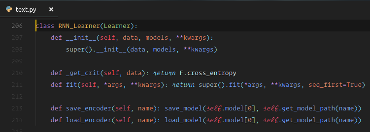
We could just call Learner to turn that into a learner, but if we call RNN_Learner, it does add in save_encoder and load_encoder that can be handy sometimes. In this case, we really could have said Leaner but RNN_Learner also works.

# Find the learning rate
learn.lr_find()
learn.sched.plot()

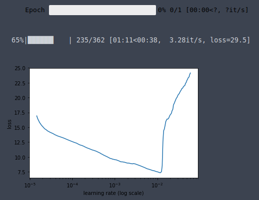
# Fit the model (15-20 mins to train)
lr = 3e-3
learn.fit(lr, 1, cycle_len=12, use_clr=(20, 10))

# -----------------------------------------------------------------------------
# Output
# -----------------------------------------------------------------------------
epoch      trn_loss   val_loss
    0      5.209042   5.980303
    1      4.513244   4.566818
    2      4.056711   4.515142
    3      3.775803   4.026515
    4      3.595237   3.857968
    5      3.519258   3.773164
    6      3.160189   3.705156
    7      3.108818   3.66531
    8      3.142783   3.613333
    9      3.192778   3.680305
    10     2.844773   3.637095
    11     2.857365   3.5963
[array([3.5963])]

learn.save('initial')
learn.load('initial')

It took me ~2 minutes (109.80s) to train 1 epoch on K80, roughly 3.35 iteration/s. The full training took me ~20 minutes.

Test [01:11:01]

Remember the model attribute of a learner is a standard PyTorch model so we can pass some x which we can grab out of our validation set or you could learn.predict_array or whatever you like to get some predictions. Then we convert those predictions into words by going .max()[1] to grab the index of the highest probability words to get some predictions. Then we can go through a few examples and print out the French, the correct English, and the predicted English for things that are not padding.

x, y = next(iter(val_dl))
probs = learn.model(V(x))
preds = to_np(probs.max(2)[1])

for i in range(180, 190):
    print(' '.join([ fr_itos[o] for o in x[:, i] if o != 1 ]))
    print(' '.join([ en_itos[o] for o in y[:, i] if o != 1 ]))
    print(' '.join([ en_itos[o] for o in preds[:, i] if o != 1 ]))
    print()

# -----------------------------------------------------------------------------
# Output
# -----------------------------------------------------------------------------
quelles composantes des différents aspects de la performance devraient être mesurées , quelles données pertinentes recueillir et comment ? _eos_
which components within various performance areas should be measured , whatkinds of data are appropriate to collect , and how should this be done ? _eos_
what aspects of the and and be be be be be be be be be ? ? _eos_

le premier ministre doit - il nommer un ministre d' état à la santé mentale , à la maladie mentale et à la toxicomanie ? _eos_
what role can the federal government play to ensure that individuals with mental illness and addiction have access to the drug therapy they need ? _eos_
what minister the minister minister minister minister minister , , , , health health and health ? ? ? ? _eos_

quelles sont les conséquences de la hausse des formes d' emploi non conformes aux normes chez les travailleurs hautement qualifiés et chez ceux qui occupent des emplois plus marginaux ? _eos_
what is the impact of growing forms of non - standard employment for highly skilled workers and for those employed in more marginal occupations ? _eos_
what are the consequences of workers workers workers workers workers workers and and workers and workers workers workers workers workers workers ? ? ? _eos_ _eos_

que se produit - il si le gestionnaire n' est pas en mesure de donner à l' employé nommé pour une période déterminée un préavis de cessation d' emploi d' un mois ou s' il néglige de le
what happens if the manager is unable to or neglects to give a term employee the one - month notice of non - renewal ? _eos_
what happens the the employee employee employee employee employee the the the the the or or the the the ? ? _eos_

quelles personnes , communautés ou entités sont considérées comme potentiels i ) bénéficiaires de la protection et ii ) titulaires de droits ? _eos_
which persons , communities or entities are identified as potential ( i ) beneficiaries of protection and / or ( ii ) rights holders ? _eos_
who , , , , , or or or or or or or or protection ? ? ? ? _eos_

quelles conditions particulières doivent être remplies pendant l' examen préliminaire international en ce qui concerne les listages des séquences de nucléotides ou d' acides aminés ou les tableaux y relatifs ? _eos_
what special requirements apply during the international preliminary examination to nucleotide and / or amino acid sequence listings and / or tables related thereto ? _eos_
what specific must be be be be sequence sequence or or or or sequence or or sequence or sequence or sequence in in ? ? ? ? _eos_ _eos_

pourquoi cette soudaine réticence à promouvoir l' égalité des genres et à protéger les femmes de ce que , dans la plupart des cas , on peut qualifier de violations grossières des droits humains ? _eos_
why this sudden reluctance to effectively promote gender equality and protect women from what are – in many cases – egregious human rights violations ? _eos_
why is the so for such of of of of of and rights and rights rights of rights rights ? ? ? ? _eos_ _eos_

pouvez - vous dire comment votre bagage culturel vous a aidée à aborder votre nouvelle vie au canada ( à vous adapter au mode de vie canadien ) ? _eos_
what are some things from your cultural background that have helped you navigate canadian life ( helped you adjust to life in canada ) ? _eos_
what are you new to to to to to to to to life life life life ? ? ? ? _eos_ _eos_

selon vous , quels seront , dans les dix prochaines années , les cinq enjeux les plus urgents en matière d' environnement et d' avenir viable pour vous et votre région ? _eos_
which do you think will be the five most pressing environmental and sustainability issues for you and your region in the next ten years ? _eos_
what do you see the next priorities priorities next the next the and and in in in in in in ? ? ? ? ? _eos_ _eos_

dans quelle mesure l' expert est-il motivé et capable de partager ses connaissances , et dans quelle mesure son successeur est-il motivé et capable de recevoir ce savoir ? _eos_
what is the expert 's level of motivation and capability for sharing knowledge , and the successor 's motivation and capability of acquiring it ? _eos_
what is the nature and and and and and and and and and and and and and to to to ? ? ? ? _eos_ _eos_ _eos_

Amazingly enough, this kind of simplest possible written largely from scratch PyTorch module on only fifty thousand sentences is sometimes capable, on validation set, of giving you exactly the right answer. Sometimes the right answer is in slightly different wording, and sometimes sentences that really aren't grammatically sensible or even have too many question marks. So we are well on the right track. We think you would agree even the simplest possible seq-to-seq trained for a very small number of epochs without any pre-training other than the use of word embeddings is surprisingly good. We are going to improve this later but the message here is even sequence to sequence models you think is simpler than they could possibly work even with less data than you think you could learn from can be surprisingly effective and in certain situations this may be enough for your needs.

❓ Would it help to normalize punctuation (e.g. ' vs. ')? [01:13:10]

The answer to this particular case is probably yes — the difference between curly quotes and straight quotes is really semantic. You do have to be very careful though because it may turn out that people using beautiful curly quotes like using more formal language and they are writing in a different way. So if you are going to do some kind of pre-processing like punctuation normalization, you should definitely check your results with and without because nearly always that kind of pre-processing make things worse even when you're sure it won't.

❓ What might be some ways of regularizing these seq2seq models besides dropout and weight decay? [01:14:17]

🔖 Let me think about that during the week. AWD-LSTM which we have been relying a lot has dropouts of many different kinds and there is also a kind of a regularization based on activations and on changes. Jeremy has not seen anybody put anything like that amount of work into regularizing sequence to sequence model and there is a huge opportunity for somebody to do like the AWD-LSTM of seq-to-seq which might be as simple as stealing all the ideas from AWD-LSTM and using them directly in seq-to-seq that would be pretty easy to try. There's been an interesting paper that Stephen Merity added in the last couple weeks where he used an idea which take all of these different AWD-LSTM hyper parameters and train a bunch of different models and then use a random forest to find out the feature importance — which ones actually matter the most and then figure out how to set them. You could totally use this approach to figure out for sequence to sequence regularization approaches which one is the best and optimize them and that would be amazing. But at the moment, we don't know if there are additional ideas to sequence to sequence regularization beyond what is in that paper for regular language model.

Tricks [01:16:28]

Trick #1 : Go bi-directional

For classification, the approach to bi-directional Jeremy suggested to use is take all of your token sequences, spin them around, train a new language model, and train a new classifier. He also mentioned that WikiText pre-trained model if you replace fwd with bwd in the name, you will get the pre-trained backward model he created for you. Get a set of predictions and then average the predictions just like a normal ensemble. That is how we do bi-dir for that kind of classification. There may be ways to do it end-to-end, but Jeremy hasn't quite figured them out yet and they are not in fastai yet. So if you figure it out, that's an interesting line of research. But because we are not doing massive documents where we have to chunk it into separate bits and then pool over them, we can do bi-dir very easily in this case. It is literally as simple as adding bidirectional = True to our encoder. People tend not to do bi-directional for the decoder partly because it is kind of considered cheating but maybe it can work in some situations although it might need to be more of an ensemble approach in the decoder because it's a bit less obvious. But encoder it's very simple — bidirectional = True and we now have a second RNN that is going the opposite direction. The second RNN is visiting each token in the opposing order so when we get to the final hidden state, it is the first (i.e. left most) token . But the hidden state is the same size, so the final result is that we end up with a tensor with an extra axis of length 2. Depending on what library you use, often that will be then combined with the number of layers, so if you have 2 layers and bi-directional — that tensor dimension is now length 4. With PyTorch it depends which bit of the process you are looking at as to whether you get a separate result for each layer and/or for each bidirectional bit. You have to look up the documentation and it will tell you input's output's tensor sizes appropriate for the number of layers and whether you have bidirectional = True.

In this particular case, you will see all the changes that had to be made [01:19:38]. For example ,when we added bidirectional = True, the Linear layer now needs number of hidden times 2 (i.e. nh * 2) to reflect the fact that we have that second direction in our hidden state. Also in initHidden it's now self.nl * 2.

class Seq2SeqRNN_Bidir(nn.Module):
    def __init__(self, vecs_enc, itos_enc, em_sz_enc, vecs_dec, itos_dec, em_sz_dec, nh, out_sl, nl=2):
        super().__init__()
        self.nl, self.nh, self.out_sl = nl, nh, out_sl
        self.emb_enc = create_emb(vecs_enc, itos_enc, em_sz_enc)
        self.emb_enc_drop = nn.Dropout(0.15)
        self.gru_enc = nn.GRU(em_sz_enc, nh, num_layers=nl, dropout=0.25, bidirectional=True) # for bidir, bidirectional=True
        self.out_enc = nn.Linear(nh * 2, em_sz_dec, bias=False) # for bidir, nh * 2
        self.drop_enc = nn.Dropout(0.05) # additional for bidir

        self.emb_dec = create_emb(vecs_dec, itos_dec, em_sz_dec)
        self.gru_dec = nn.GRU(em_sz_dec, em_sz_dec, num_layers=nl, dropout=0.1)
        self.out_drop = nn.Dropout(0.35)
        self.out = nn.Linear(em_sz_dec, len(itos_dec))
        self.out.weight.data = self.emb_dec.weight.data

    def forward(self, inp):
        sl, bs = inp.size()

        # ==================================================
        # Encoder version
        # ==================================================

        h = self.initHidden(bs)
        emb = self.emb_enc_drop(self.emb_enc(inp))
        enc_out, h = self.gru_enc(emb, h)
        # Additional for bidir
        h = h.view(2, 2, bs, -1).permute(0, 2, 1, 3).contiguous().view(2, bs, -1)
        h = self.out_enc(self.drop_enc(h)) # new for bidir; dropout hidden state.

        # ==================================================
        # Decoder version
        # ==================================================

        dec_inp = V(torch.zeros(bs).long())
        res = []

        for i in range(self.out_sl):
            emb = self.emb_dec(dec_inp).unsqueeze(0)
            outp, h = self.gru_dec(emb, h)
            outp = self.out(self.out_drop(outp[0]))
            res.append(outp)
            dec_inp = V(outp.data.max(1)[1])

            if (dec_inp == 1).all():
                break

        return torch.stack(res)

    def initHidden(self, bs):
        return V(torch.zeros(self.nl * 2, bs, self.nh)) # for bidir, sel.nl * 2

rnn = Seq2SeqRNN_Bidir(fr_vecd, fr_itos, dim_fr_vec, en_vecd, en_itos, dim_en_vec, nh, enlen_90)
learn = RNN_Learner(md, SingleModel(to_gpu(rnn)), opt_fn=opt_fn)
learn.crit = seq2seq_loss

learn.fit(lr, 1, cycle_len=12, use_clr=(20, 10))

# -----------------------------------------------------------------------------
# Output
# -----------------------------------------------------------------------------
epoch      trn_loss   val_loss
    0      4.766771   4.495123
    1      3.918195   4.018911
    2      3.682928   3.852527
    3      3.654867   3.653316
    4      3.540806   3.581977
    5      3.38937    3.518663
    6      3.337964   3.461221
    7      2.868424   3.439734
    8      2.783658   3.426322
    9      2.743709   3.375462
    10     2.662714   3.39351
    11     2.551906   3.373751
[array([3.37375])]

It took me ~2 minutes (115.30s) to train 1 epoch on K80, roughly 3.10 iteration/s. The full training took me ~23 minutes.

❓ Why is making the decoder bi-directional considered cheating? [01:20:13]

It's not just cheating but we have this loop going on so it is not as simple as having two tensors. Then how do you turn those two separate loops into a final result? After talking about it during the break, Jeremy has gone from "everybody knows it doesn't work" to "maybe it could work", but it requires more thought. It is quite possible during the week, he'll realize it's a dumb idea, but we'll think about it.

❓ Why do you need to set a range to the loop? [01:20:58]

Because when we start training, everything is random so if (dec_inp == 1).all(): break will probably never be true. Later on, it will pretty much always break out eventually but basically we are going to go forever. It's really important to remember when you are designing an architecture that when you start, the model knows nothing about anything. So you want to make sure if it's going to do something at least it's vaguely sensible.

We got 3.5963 cross entropy loss with single direction [01:21:46]. With bi-direction, we got down to 3.37375, so that improved a little. It shouldn't really slow things down too much. Bi-directional does mean there is a little bit more sequential processing have to happen, but it is generally a good win. In the Google translation model, of the 8 layers, only the first layer is bi-directional because it allows it to do more in parallel, so if you create really deep models you may need to think about which ones are bi-directional otherwise we have performance issues.

Trick #2 Teacher Forcing [01:22:39]

Now let's talk about teacher forcing. When a model starts learning, it knows nothing about nothing. So when the model starts learning, it is not going to spit out "Er" at the first step, it is going to spit out some random meaningless word because it doesn't know anything about German or about English or about the idea of language. And it is going to feed it to the next process as an input and be totally unhelpful. That means, early learning is going to be very difficult because it is feeding in an input that is stupid into a model that knows nothing and somehow it's going to get better. So it is not asking too much eventually it gets there, but it's definitely not as helpful as we can be. So what if instead of feeing in the thing I predicted just now, what if we instead we feed in the actual correct word was meant to be. We can't do that at inference time because by definition we don't know the correct word - it has to translate it. We can't require the correct translation in order to do translation.

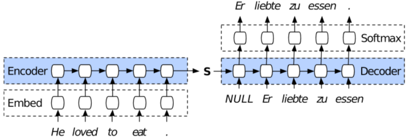
So the way it's set up is we have this thing called pr_force which is probability of forcing [01:24:01]. If some random number is less than that probability then we are going to replace our decoder input with the actual correct thing. If we have already gone too far and if it is already longer than the target sequence, we are just going to stop because obviously we can't give it the correct thing. So you can see how beautiful PyTorch is for this. The key reasons that we switched to PyTorch at this exact point in last year's class was because Jeremy tried to implement teacher forcing in Keras and TensorFlow and went even more insane than he started. It was weeks of getting nowhere then he saw on Twitter Andrej Karpathy said something about this thing called PyTorch that just came out and it's really cool. He tried it that day, by the next day, he had teacher forcing. All this stuff of trying to debug things was suddenly so much easier and and this kind of dynamic thing is so much easier. So this is a great example of "hey, I get to use random numbers and if statements".

class Seq2SeqStepper(Stepper):
    def step(self, xs, y, epoch):
        self.m.pr_force = (10 - epoch) * 0.1 if epoch < 10 else 0
        xtra = []
        output = self.m(*xs, y)
        if isinstance(output, tuple):
            output, *xtra = output
        self.opt.zero_grad()
        loss = raw_loss = self.crit(output, y)
        if self.reg_fn:
            loss = self.reg_fn(output, xtra, raw_loss)
        loss.backward()
        if self.clip: # gradient clipping
            nn.utils.clip_grad_norm(trainable_params_(self.m), self.clip)
        self.opt.step()

        return raw_loss.data[0]

Here is the basic idea [01:25:29]. At the start of training, let's set pr_force really high so that nearly always it gets the actual correct previous word and so it has a useful input. Then as we trained a bit more, let's decrease pr_force so that by the end pr_force is zero and it has to learn properly which is fine because it is now actually feeding in sensible inputs most of the time anyway.

class Seq2SeqRNN_TeacherForcing(nn.Module):
    def __init__(self, vecs_enc, itos_enc, em_sz_enc, vecs_dec, itos_dec, em_sz_dec, nh, out_sl, nl=2):
        super().__init__()
        self.nl, self.nh, self.out_sl = nl, nh, out_sl
        self.emb_enc = create_emb(vecs_enc, itos_enc, em_sz_enc)
        self.emb_enc_drop = nn.Dropout(0.15)
        self.gru_enc = nn.GRU(em_sz_enc, nh, num_layers=nl, dropout=0.25)
        self.out_enc = nn.Linear(nh, em_sz_dec, bias=False)
        self.emb_dec = create_emb(vecs_dec, itos_dec, em_sz_dec)
        self.gru_dec = nn.GRU(em_sz_dec, em_sz_dec, num_layers=nl, dropout=0.1)
        self.out_drop = nn.Dropout(0.35)
        self.out = nn.Linear(em_sz_dec, len(itos_dec))
        self.out.weight.data = self.emb_dec.weight.data
        self.pr_force = 1. # new for teacher forcing

    def forward(self, inp, y=None): # argument y is new for teacher forcing
        sl, bs = inp.size()
        h = self.initHidden(bs)
        emb = self.emb_enc_drop(self.emb_enc(inp))
        enc_out, h = self.gru_enc(emb, h)
        h = self.out_enc(h)

        dec_inp = V(torch.zeros(bs).long())
        res = []

        for i in range(self.out_sl):
            emb = self.emb_dec(dec_inp).unsqueeze(0)
            outp, h = self.gru_dec(emb, h)
            outp = self.out(self.out_drop(outp[0]))
            res.append(outp)
            dec_inp = V(outp.data.max(1)[1])

            if (dec_inp == 1).all():
                break
            if (y is not None) and (random.random() < self.pr_force): # new for teacher forcing
                if i >= len(y):
                    break
                dec_inp = y[i]
        return torch.stack(res)

    def initHidden(self, bs):
        return V(torch.zeros(self.nl, bs, self.nh))

pr_force: "probability of forcing". High in the beginning zero by the end.

Let's now write something such that in the training loop, it gradually decreases pr_force [01:26:01]. How do we do that? One approach would be to write our own training loop but let's not do that because we already have a training loop that has progress bars, uses exponential weighted averages to smooth out the losses, keeps track of metrics, and does bunch of things. They also keep track of calling the reset for RNN at the start of the epoch to make sure the hidden state is set to zeros. What we've tended to find is that as we start to write some new thing and we need to replace some part of the code, we then add some little hook so that we can all use that hook to make things easier. In this particular case, there is a hook that Jeremy has ended up using all the time which is the hook called the stepper. If you look at the source code, model.py is where our fit function lives which is the lowest level thing that does not require learner or anything much at all — just requires a standard PyTorch model and a model data object. You just need to know how many epochs, a standard PyTorch optimizer, and a standard PyTorch loss function. We hardly ever used in the class, we normally call learn.fit, but learn.fit calls this.

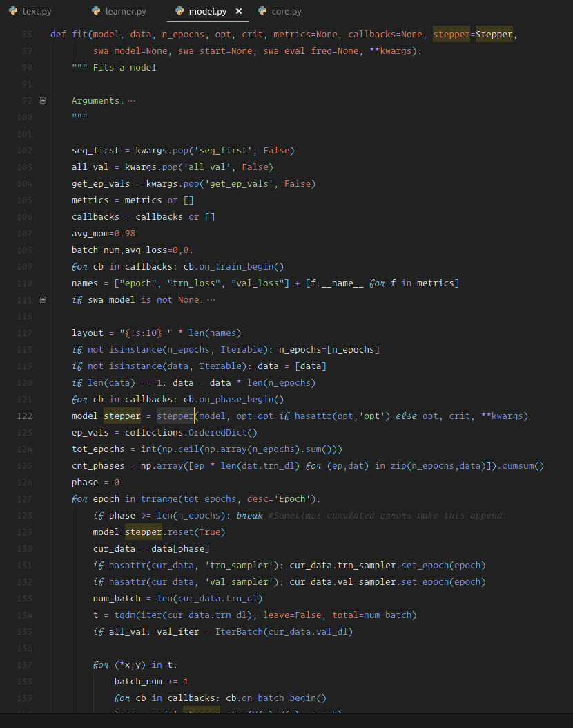
We have to look at the source code sometime [01:27:49]. We've seen how it loop through each epoch and that loops through each thing in our batch and calls stepper.step. stepper.step is the thing that is responsible for:

• calling the model
• getting the loss
• finding the loss function
• calling the optimizer

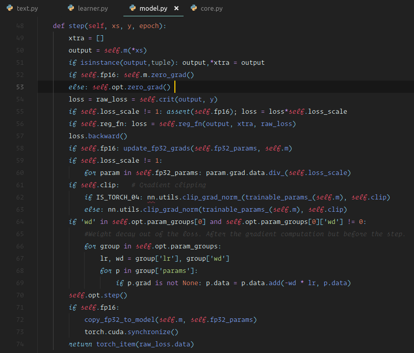
So by default, stepper.step uses a particular class called Stepper which basically calls the model, zeros the gradient, calls the loss function, calls backward, does gradient clipping if necessary, then calls the optimizer. They are basic steps that back when we looked at "PyTorch from scratch" we had to do. The nice thing is, we can replace that with something else rather than replacing the training loop. If you inherit from Stepper, then write your own version of step, you can just copy and paste the contents of step and add whatever you like. Or if it's something that you're going to do before or afterwards, you could even call super.step. In this case, Jeremy rather suspects he has been unnecessarily complicated [01:29:12] — he probably could have done something like:

class Seq2SeqStepper(Stepper):
    def step(self, xs, y, epoch):
        self.m.pr_force = (10 - epoch) * 0.1 if epoch < 10 else 0
        return super.step(xs, y, epoch)

But as he said, when he is prototyping, he doesn't think carefully about how to minimize his code — he copied and pasted the contents of the step and he added a single line to the top which was to replace pr_force in the module with something that gradually decreased linearly for the first 10 epochs, and after 10 epochs, it is zero. So total hack but good enough to try it out. The nice thing is that everything else is the same except for the addition of these three lines:

if (y is not None) and (random.random() < self.pr_force):
    if i >= len(y): break
    dec_inp = y[i]

And the only thing we need to do differently is when we call fit, we pass in our customized stepper class.

rnn = Seq2SeqRNN_TeacherForcing(fr_vecd, fr_itos, dim_fr_vec, en_vecd, en_itos, dim_en_vec, nh, enlen_90)
learn = RNN_Learner(md, SingleModel(to_gpu(rnn)), opt_fn=opt_fn)
learn.crit = seq2seq_loss

learn.fit(lr, 1, cycle_len=12, use_clr=(20, 10), stepper=Seq2SeqStepper)

# -----------------------------------------------------------------------------
# Output
# -----------------------------------------------------------------------------
epoch      trn_loss   val_loss
    0      3.972275   11.894288
    1      3.75144    8.904335
    2      3.147096   5.737202
    3      3.205919   4.434411
    4      2.89941    4.337346
    5      2.837049   4.195613
    6      2.9374     3.801485
    7      2.919509   3.679037
    8      2.974855   3.600216
    9      2.98231    3.551779
    10     2.871864   3.418646
    11     2.674465   3.432893
[array([3.43289])]

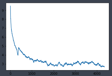
It took me ~1 minute (78.62s) to train 1 epoch on K80, roughly 5.0 iteration/s. The full training took me ~16 minutes.

And now our loss is down to 3.43. We needed to make sure at least do 10 epochs because before that, it was cheating by using the teacher forcing.

Trick #3 Attentional model [01:31:00]

This next trick is a bigger and pretty cool trick. It's called "attention." The basic idea of attention is this — expecting the entirety of the sentence to be summarized into this single hidden vector is asking a lot. It has to know what was said, how it was said, and everything necessary to create the sentence in German. The idea of attention is basically maybe we are asking too much. Particularly because we could use this form of model (below) where we output every step of the loop to not just have a hidden state at the end but to have a hidden state after every single word. Why not try and use that information? It's already there but so far we've just been throwing it away. Not only that but bi-directional, we got two vectors of state every step that we can use. How can we do this?

Let's say we are translating a word "liebte" right now [01:32:34]. Which of previous 5 pieces of state do we want? We clearly want "love" because it is the word. How about "zu"? We probably need "eat" and "to" and loved" to make sure we have gotten the tense right and know that I actually need this part of the verb and so forth. So depending on which bit we are translating, we would need one or more bits of these various hidden states. In fact, we probably want some weighting of them. In other words, for these five pieces of hidden state, we want a weighted average [01:33:47]. We want it weighted by something that can figure out which bits of the sentence is the most important right now. How do we figure out something like which bits of the sentence are important right now? We create a neural net and we train the neural net to figure it out. When do we train that neural net? End to end. So let's now train two neural nets [01:34:18]. Well, we've already got a bunch — RNN encoder, RNN decoder, a couple of linear layers, what the heck, let's add another neural net into the mix. This neural net is going to spit out a weight for every one of these states and we will take the weighted average at every step, and it's just another set of parameters that we learn all at the same time. So that is called "attention".

The idea is that once that attention has been learned, each word is going to take a weighted average as you can see in this terrific demo from Chris Olah and Shan Carter [01:34:50]. Check out this distill.pub article — these things are interactive diagrams that shows you how the attention works and what the actual attention looks like in a trained translation model.

Let's try and implement attention [01:35:47]:

def rand_t(*sz):
    return torch.randn(sz) / math.sqrt(sz[0])

def rand_p(*sz):
    return nn.Parameter(rand_t(*sz))

class Seq2SeqAttnRNN(nn.Module):
    def __init__(self, vecs_enc, itos_enc, em_sz_enc, vecs_dec, itos_dec, em_sz_dec, nh, out_sl, nl=2):
        super().__init__()
        self.emb_enc = create_emb(vecs_enc, itos_enc, em_sz_enc)
        self.nl,self.nh,self.out_sl = nl,nh,out_sl
        self.gru_enc = nn.GRU(em_sz_enc, nh, num_layers=nl, dropout=0.25)
        self.out_enc = nn.Linear(nh, em_sz_dec, bias=False)
        self.emb_dec = create_emb(vecs_dec, itos_dec, em_sz_dec)
        self.gru_dec = nn.GRU(em_sz_dec, em_sz_dec, num_layers=nl, dropout=0.1)
        self.emb_enc_drop = nn.Dropout(0.15)
        self.out_drop = nn.Dropout(0.35)
        self.out = nn.Linear(em_sz_dec, len(itos_dec))
        self.out.weight.data = self.emb_dec.weight.data

        # these 4 lines are addition for 'attention'
        self.W1 = rand_p(nh, em_sz_dec) # random matrix
        self.l2 = nn.Linear(em_sz_dec, em_sz_dec) # this is the mini NN that will calculate the weights
        self.l3 = nn.Linear(em_sz_dec + nh, em_sz_dec)
        self.V = rand_p(em_sz_dec)

    def forward(self, inp, y=None, ret_attn=False):
        sl, bs = inp.size()
        h = self.initHidden(bs)
        emb = self.emb_enc_drop(self.emb_enc(inp))
        enc_out, h = self.gru_enc(emb, h)
        h = self.out_enc(h)

        dec_inp = V(torch.zeros(bs).long())
        res, attns = [], [] # attns is addition for 'attention'
        w1e = enc_out @ self.W1 # this line is addition for 'attention'. matrix multiply.

        for i in range(self.out_sl):
            # these 5 lines are addition for 'attention'.

            # create a little neural network.
            # use softmax to generate the probabilities.
            w2h = self.l2(h[-1]) # take last layers hidden state put into linear layer
            u = F.tanh(w1e + w2h) # nonlinear activation
            a = F.softmax(u @ self.V, 0) # matrix multiply
            attns.append(a)
            # take a weighted average. Use the weights from mini NN.
            # note we are using all the encoder states
            Xa = (a.unsqueeze(2) * enc_out).sum(0)

            emb = self.emb_dec(dec_inp)
            # adding the hidden states to the encoder weights
            wgt_enc = self.l3(torch.cat([emb, Xa], 1)) # this line is addition for 'attention'

            outp, h = self.gru_dec(wgt_enc.unsqueeze(0), h) # this line has changed for 'attention'
            outp = self.out(self.out_drop(outp[0]))
            res.append(outp)
            dec_inp = V(outp.data.max(1)[1])
            if (dec_inp==1).all():
                break
            if (y is not None) and (random.random() < self.pr_force): # why is teacher forcing logic still here? bug?
                if i >= len(y):
                    break
                dec_inp = y[i]

        res = torch.stack(res)
        if ret_attn:
            res = torch.stack(attns) # bug? fixed!
        return res

    def initHidden(self, bs):
        return V(torch.zeros(self.nl, bs, self.nh))

With attention, most of the code is identical. The one major difference is this line: Xa = (a.unsqueeze(2) * enc_out).sum(0). We are going to take a weighted average and the way we are going to do the weighted average is we create a little neural net which we are going to see here:

w2h = self.l2(h[-1])
u = F.tanh(w1e + w2h)
a = F.softmax(u @ self.V, 0)

We use softmax because the nice thing about softmax is that we want to ensure all of the weights that we are using add up to 1 and we also expect that one of those weights should probably be higher than the other ones [01:36:38]. Softmax gives us the guarantee that they add up to 1 and because it has e^ in it, it tends to encourage one of the weights to be higher than the other ones.

Let's see how this works [01:37:09]. We are going to take the last layer's hidden state and we are going to stick it into a linear layer. Then we are going to stick it into a nonlinear activation, then we are going to do a matrix multiply. So if you think about it — a linear layer, nonlinear activation, matrix multiply — it's a neural net. It is a neural net with one hidden layer. Stick it into a softmax and then we can use that to weight our encoder outputs. Now rather than just taking the last encoder output, we have the whole tensor of all of the encoder outputs which we just weight by this neural net we created.

In Python, A @ B is the matrix product, A * B the element-wise product.

Papers [01:38:18]

• Neural Machine Translation by Jointly Learning to Align and Translate—One amazing paper that originally introduced this idea of attention as well as a couple of key things which have really changed how people work in this field. They say area of attention has been used not just for text but for things like reading text out of pictures or doing various things with computer vision.
• Grammar as a Foreign Language —The second paper which Geoffrey Hinton was involved in that used this idea of RNN with attention to try to replace rules based grammar with an RNN which automatically tagged each word based on the grammar. It turned out to do it better than any rules based system which today seems obvious but at that time it was considered really surprising. They are summary of how attention works which is really nice and concise.

❓ Could you please explain attention again? [01:39:46]

Sure! Let's go back and look at our original encoder.

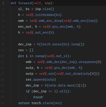
The RNN spits out two things: it spits out a list of the state after every time step (enc_out), and it also tells you the state at the last time step (h)and we used the state at the last time step to create the input state for our decoder which is one vector s below:

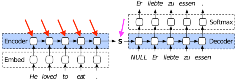
But we know that it's creating a vector at every time steps (orange arrows), so wouldn't it be nice to use them all? But wouldn't it be nice to use the one or ones that's most relevant to translating the word we are translating now? So wouldn't it be nice to be able to take a weighted average of the hidden state at each time step weighted by whatever is the appropriate weight right now. For example, "liebte" would definitely be time step #2 is what it's all about because that is the word I'm translating. So how do we get a list of weights that is suitable for the word we are training right now? The answer is by training a neural net to figure out the list of weights. So anytime we want to figure out how to train a little neural net that does any task, the easiest way, normally always to do that is to include it in your module and train it in line with everything else. The minimal possible neural net is something that contains two layers and one nonlinear activation function, so self.l2 is one linear layer.

In fact, instead of a linear layer, we can even just grab a random matrix if we do not care about bias [01:42:18]. self.W1 is a random tensor wrapped up in a Parameter.

Parameter : Remember, a Parameter is identical to PyTorch Variable but it just tells PyTorch "I want you to learn the weights for this please." [01:42:35]

So when we start out our decoder, let's take the current hidden state of the decoder, put that into a linear layer (self.l2) because what is the information we use to decide what words we should focus on next — the only information we have to go on is what the decoder's hidden state is now. So let's grab that:

• put it into the linear layer (self.l2)
• put it through a non-linearity (F.tanh)
• put it through one more nonlinear layer (u @ self.V doesn't have a bias in it so it's just matrix multiply)
• put that through softmax

That's it — a little neural net. It doesn't do anything. It's just a neural net and no neural nets do anything they are just linear layers with nonlinear activations with random weights. But it starts to do something if we give it a job to do. In this case, the job we give it to do is to say don't just take the final state but now let's use all of the encoder states and let's take all of them and multiply them by the output of that little neural net. So given that the things in this little neural net are learnable weights, hopefully it's going to learn to weight those encoder hidden states by something useful. That is all neural net ever does is we give it some random weights to start with and a job to do, and hope that it learns to do the job. It turns out, it does.

Everything else in here is identical to what it was before. We have teacher forcing, it's not bi-directional, so we can see how this goes.

rnn = Seq2SeqAttnRNN(fr_vecd, fr_itos, dim_fr_vec, en_vecd, en_itos, dim_en_vec, nh, enlen_90)
learn = RNN_Learner(md, SingleModel(to_gpu(rnn)), opt_fn=opt_fn)
learn.crit = seq2seq_loss

lr = 2e-3

learn.fit(lr, 1, cycle_len=15, use_clr=(20, 10), stepper=Seq2SeqStepper)

# -----------------------------------------------------------------------------
# Output
# -----------------------------------------------------------------------------
epoch      trn_loss   val_loss
    0      3.780541   14.757052
    1      3.221531   5.661915
    2      2.901307   4.924356
    3      2.875144   4.647381
    4      2.704298   3.912943
    5      2.69899    4.401953
    6      2.78165    3.864044
    7      2.765688   3.614325
    8      2.873574   3.417437
    9      2.826172   3.370511
    10     2.845763   3.293398
    11     2.66649    3.300835
    12     2.697862   3.258844
    13     2.659374   3.267969
    14     2.585613   3.240595
[array([3.24059])]

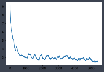
It took me ~1 min 22s (82.42s) to train 1 epoch on K80, roughly 4.65 iteration/s. The full training took me ~25 minutes.

Teacher forcing had 3.49 and now with nearly exactly the same thing but we've got this little minimal neural net figuring out what weightings to give our inputs and we are down to 3.37. Remember, these loss are logs, so e^3.37 is quite a significant change.

x, y = next(iter(val_dl))
probs, attns = learn.model(V(x), ret_attn=True)
preds = to_np(probs.max(2)[1])

for i in range(180, 190):
    print(' '.join([fr_itos[o] for o in x[:, i] if o != 1]))
    print(' '.join([en_itos[o] for o in y[:, i] if o != 1]))
    print(' '.join([en_itos[o] for o in preds[:, i] if o != 1]))
    print()

# -----------------------------------------------------------------------------
# Output
# -----------------------------------------------------------------------------
quelles composantes des différents aspects de la performance devraient être mesurées , quelles données pertinentes recueillir et comment ? _eos_
which components within various performance areas should be measured , whatkinds of data are appropriate to collect , and how should this be done ? _eos_
what components of the performance should be be be data be and and how ? ? _eos_ ?

le premier ministre doit - il nommer un ministre d' état à la santé mentale , à la maladie mentale et à la toxicomanie ? _eos_
what role can the federal government play to ensure that individuals with mental illness and addiction have access to the drug therapy they need ? _eos_
what is the minister minister 's minister minister to to minister to health health ? and mental mental health _eos_ _eos_ mental _eos_

quelles sont les conséquences de la hausse des formes d' emploi non conformes aux normes chez les travailleurs hautement qualifiés et chez ceux qui occupent des emplois plus marginaux ? _eos_
what is the impact of growing forms of non - standard employment for highly skilled workers and for those employed in more marginal occupations ? _eos_
what are the implications of of - statistics - workers - workers workers and and skilled workers workers workers older workers _eos_ ? workers ? _eos_ _eos_

que se produit - il si le gestionnaire n' est pas en mesure de donner à l' employé nommé pour une période déterminée un préavis de cessation d' emploi d' un mois ou s' il néglige de le
what happens if the manager is unable to or neglects to give a term employee the one - month notice of non - renewal ? _eos_
what if the manager is not to to employee employee employee a employee the employee for retirement time hours employee after a employee of ? after _eos_

quelles personnes , communautés ou entités sont considérées comme potentiels i ) bénéficiaires de la protection et ii ) titulaires de droits ? _eos_
which persons , communities or entities are identified as potential ( i ) beneficiaries of protection and / or ( ii ) rights holders ? _eos_
who , or or or or considered as as recipients of of of protection protection protection _eos_ ? _eos_ _eos_

quelles conditions particulières doivent être remplies pendant l' examen préliminaire international en ce qui concerne les listages des séquences de nucléotides ou d' acides aminés ou les tableaux y relatifs ? _eos_
what special requirements apply during the international preliminary examination to nucleotide and / or amino acid sequence listings and / or tables related thereto ? _eos_
what specific conditions conditions be be during the international examination examination in the for nucleotide or amino amino / or or ? _eos_ ? ? _eos_ tables _eos_ ?

pourquoi cette soudaine réticence à promouvoir l' égalité des genres et à protéger les femmes de ce que , dans la plupart des cas , on peut qualifier de violations grossières des droits humains ? _eos_
why this sudden reluctance to effectively promote gender equality and protect women from what are – in many cases – egregious human rights violations ? _eos_
why this this to to to to to to women to and and and women to , of _eos_ of many people ? ? of _eos_ ? human human

pouvez - vous dire comment votre bagage culturel vous a aidée à aborder votre nouvelle vie au canada ( à vous adapter au mode de vie canadien ) ? _eos_
what are some things from your cultural background that have helped you navigate canadian life ( helped you adjust to life in canada ) ? _eos_
what is your your of your you to you to to in canada canada canada life canada canada canada _eos_ _eos_ _eos_ _eos_ _eos_

selon vous , quels seront , dans les dix prochaines années , les cinq enjeux les plus urgents en matière d' environnement et d' avenir viable pour vous et votre région ? _eos_
which do you think will be the five most pressing environmental and sustainability issues for you and your region in the next ten years ? _eos_
what do you think in the next five five next , , next and and and and and and you and in ? _eos_ ? ? _eos_ ?

dans quelle mesure l' expert est-il motivé et capable de partager ses connaissances , et dans quelle mesure son successeur est-il motivé et capable de recevoir ce savoir ? _eos_
what is the expert 's level of motivation and capability for sharing knowledge , and the successor 's motivation and capability of acquiring it ? _eos_
what is the the of the the and and and and and and and to and to and and ? ? ? _eos_ _eos_

Not bad. It's still not perfect but quite a few of them are correct and again considering that we are asking it to learn about the very idea of language for two different languages and how to translate them between the two, and grammar, and vocabulary, and we only have 50,000 sentences and a lot of the words only appear once, I would say this is actually pretty amazing.

❓ Why do we use tanh instead of ReLU for the attention mini net? [01:46:23]

I don't quite remember — it's been a while since I looked at it. You should totally try using value and see how it goes. Obviously tanh the key difference is that it can go in each direction and it's limited both at the top and the bottom. I know very often for the gates inside RNNs, LSTMs, and GRUs, tanh often works out better but it's been about a year since I actually looked at that specific question so I'll look at it during the week. The short answer is you should try a different activation function and see if you can get a better result.

From Lesson 7 [00:44:06]: As we have seen last week, tanh is forcing the value to be between -1 and 1. Since we are multiplying by this weight matrix again and again, we would worry that relu (since it is unbounded) might have more gradient explosion problem. Having said that, you can specify RNNCell to use different nonlineality whose default is tanh and ask it to use relu if you wanted to.

Visualization [01:47:12]

What we can do also is we can grab the attentions out of the model by adding return attention parameter to forward function. You can put anything you'd like in forward function argument. So we added a return attention parameter, false by default because obviously the training loop it doesn't know anything about it but then we just had something here says if return attention, then stick the attentions on as well (if ret_attn: res = res,torch.stack(attns)). The attentions is simply the value a just chuck it on a list (attns.append(a)). We can now call the model with return attention equals true and get back the probabilities and the attentions [01:47:53]:

probs, attns = learn.model(V(x), ret_attn=True)

We can now draw pictures, at each time step, of the attention.

attn = to_np(attns[..., 180])

fig, axes = plt.subplots(3, 3, figsize=(15, 10))
for i, ax in enumerate(axes.flat):
    ax.plot(attn[i])

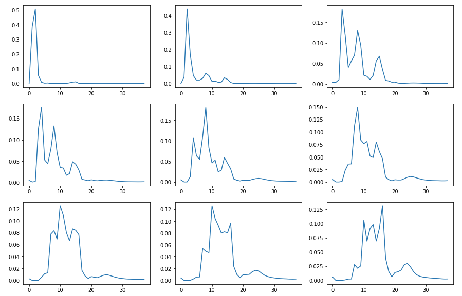
When you are Chris Olah and Shan Carter, you make things that looks like 👇 when you are Jeremy Howard, the exact same information looks like ☝️ [01:48:24]. You can see at each different time step, we have a different attention.

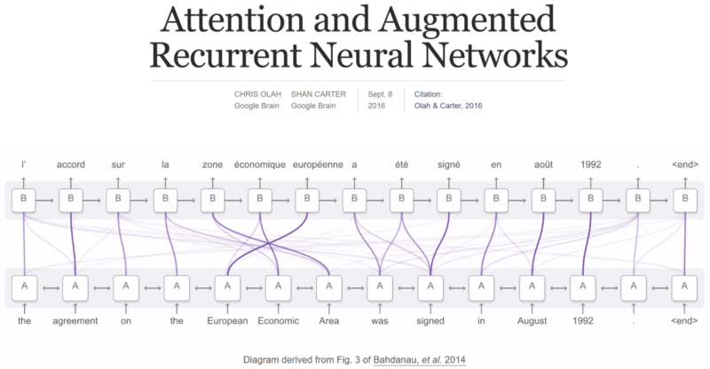
It's very important when you try to build something like this, you don't really know if it's not working right because if it's not working (as per usual Jeremy's first 12 attempts of this were broken) and they were broken in a sense that it wasn't really learning anything useful. Therefore, it was giving equal attention to everything and it wasn't worse — it just wasn't much better. Until you actually find ways to visualize the thing in a way that you know what it ought to look like ahead of time, you don't really know if it's working [01:49:16]. So it's really important that you try to find ways to check your intermediate steps in your outputs.

❓ What is the loss function of the attentional neural network? [01:49:31]

No, there is no loss function for the attentional neural network. It is trained end-to-end. It is just sitting inside our decoder loop. The loss function for the decoder loop is the same loss function because the result contains exactly same thing as before — the probabilities of the words. How come the mini neural net learning something? Because in order to make the outputs better and better, it would be great if it made the weights of weighted-average better and better. So part of creating our output is to please do a good job of finding a good set of weights and if it doesn't do a good job of finding good set of weights, then the loss function won't improve from that bit. So end-to-end learning means you throw in everything you can into one loss function and the gradients of all the different parameters point in a direction that says "hey, you know if you had put more weight over there, it would have been better." And thanks to the magic of the chain rule, it knows to put more weight over there, change the parameter in the matrix multiply a little, etc. That is the magic of end-to-end learning. It is a very understandable question but you have to realize there is nothing particular about this code that says this particular bits are separate mini neural network anymore than the GRU is a separate little neural network, or a linear layer is a separate little function. It's all ends up pushed into one output which is a bunch of probabilities which ends up in one loss function that returns a single number that says this either was or wasn't a good translation. So thanks to the magic of the chain rule, we then back propagate little updates to all the parameters to make them a little bit better. This is a big, weird, counterintuitive idea and it's totally okay if it's a bit mind-bending. It is the bit where even back to lesson 1 "how did we make it find dogs vs. cats?" — we didn't. All we did was we said "this is our data, this is our architecture, this is our loss function. Please back propagate into the weights to make them better and after you've made them better a while, it will start finding cats from dogs." In this case (i.e. translation), we haven't used somebody else's convolutional network architecture. We said "here is a custom architecture which we hope is going to be particularly good at this problem." Even without this custom architecture, it was still okay. But we made it in a way that made more sense or we think it ought to do worked even better. But at no point, did we do anything different other than say "here is a data, here is an architecture, here is a loss function — go and find the parameters please" And it did it because that's what neural nets do.

So that is sequence-to-sequence learning [01:53:19].

• If you want to encode an image into a CNN backbone of some kind, and then pass that into a decoder which is like RNN with attention, and you make your y-values the actual correct caption of each of those image, you will end up with an image caption generator.
• If you do the same thing with videos and captions, you will end up with a video caption generator.
• If you do the same thing with 3D CT scan and radiology reports, you will end up with a radiology report generator.
• If you do the same thing with Github issues and people's chosen summaries of them, you'll get a Github issue summary generator.

Seq-to-seq is magical but they work [01:54:07]. And I don't feel like people have begun to scratch the surface of how to use seq-to-seq models in their own domains. Not being a Github person, it would never have occurred to me that "it would be kind of cool to start with some issue and automatically create a summary". But now, of course, next time I go into Github, I want to see a summary written there for me. I don't want to write my own commit message. Why should I write my own summary of the code review when I finished adding comments to lots of lines — it should do that for me as well. Now I'm thinking Github so behind, it could be doing this stuff. So what are the thing in your industry? You could start with a sequence and generate something from it. I can't begin to imagine. Again, it is a fairly new area and the tools for it are not easy to use — they are not even built into fastai yet. Hopefully there will be soon. I don't think anybody knows what the opportunities are.

DeViSE [01:55:23]

devise.ipynb

We are going to do something bringing together for the first time our two little worlds we focused on — text and images [01:55:49]. This idea came up in a paper by an extraordinary deep learning practitioner and researcher named Andrea Frome. Andrea was at Google at the time and her crazy idea was words can have a distributed representation, a space, which particularly at that time was just word vectors. And images can be represented in a space. In the end, if we have a fully connected layer, they ended up as a vector representation. Could we merge the two? Could we somehow encourage the vector space that the images end up with be the same vector space that the words are in? And if we could do that, what would that mean? What could we do with that? So what could we do with that covers things like well, what if I'm wrong what if I'm predicting that this image is a beagle and I predict jumbo jet and Yannet's model predicts corgi. The normal loss function says that Yannet's and Jeremy's models are equally good (i.e. they are both wrong). But what if we could somehow say though you know what corgi is closer to beagle than it is to jumbo jets. So Yannet's model is better than Jeremy's. We should be able to do that because in word vector space, beagle and corgi are pretty close together but jumbo jet not so much. So it would give us a nice situation where hopefully our inferences would be wrong in saner ways if they are wrong. It would also allow us to search for things that are not in ImageNet Synset ID (i.e. a category in ImageNet). Why did we have to train a whole new model to find dog vs. cats when we already have something that found corgis and tabbies. Why can't we just say find me dogs? If we had trained it in word vector space, we totally could because they are word vector, we can find things with the right image vector and so forth. We will look at some cool things we can do with it in a moment but first of all let's train a model where this model is not learning a category (one hot encoded ID) where every category is equally far from every other category, let's instead train a model where we're finding a dependent variable which is a word vector. So, what is word vector? Obviously the word vector for the word you want. So if it's corgi, let's train it to create a word vector that's the corgi word vector, and if it's a jumbo jet, let's train it with a dependent variable that says this is the word vector for a jumbo jet.

from fastai.conv_learner import *
torch.backends.cudnn.benchmark = True

import fastText as ft

import torchvision.transforms as transforms

# Normalize ImageNet images
normalize = transforms.Normalize(mean=[0.485, 0.456, 0.406], std=[0.229, 0.224, 0.225])

# Image processing
tfms = transforms.Compose([
    transforms.RandomResizedCrop(224),
    transforms.RandomHorizontalFlip(),
    transforms.ToTensor(),
    normalize,
])

Download ImageNet dataset:

For me, I will use a subset of ImageNet training set this time.

%mkdir data/imagenet
%cd data/imagenet/

!aria2c --file-allocation=none -c -x 5 -s 5 http://files.fast.ai/data/imagenet-sample-train.tar.gz

!tar -xzf imagenet-sample-train.tar.gz

%cd ../..

Setup directory and file paths:

PATH = Path('data/imagenet/')
TMP_PATH = PATH / 'tmp'
TRANS_PATH = Path('data/translate/') # for fastText word vectors
PATH_TRN = PATH / 'train'

Load the Word Vectors

It is shockingly easy [01:59:17]. Let's grab the fastText word vectors again, load them in (we only need English this time).

# fastText word vectors
ft_vecs = ft.load_model(str((TRANS_PATH / 'wiki.en.bin')))

np.corrcoef( ft_vecs.get_word_vector('jeremy'), ft_vecs.get_word_vector('Jeremy') )

# -----------------------------------------------------------------------------
# Output
# -----------------------------------------------------------------------------
array([[1.     , 0.60866],
       [0.60866, 1.     ]])

So for example, "jeremy" and "Jeremy" have a correlation of .6.

np.corrcoef(ft_vecs.get_word_vector('banana'), ft_vecs.get_word_vector('Jeremy'))

# -----------------------------------------------------------------------------
# Output
# -----------------------------------------------------------------------------
array([[1.     , 0.14482],
       [0.14482, 1.     ]])

Jeremy doesn't like bananas at all, and "banana" and "Jeremy" .14. So words that you would expect to be correlated are correlated and words that should be as far away from each other as possible, unfortunately, they are still slightly correlated but not so much [01:59:41].

Map ImageNet classes to word vectors

Let's now grab all of the ImageNet classes because we actually want to know which one is corgi and which one is jumbo jet.

ft_words = ft_vecs.get_words(include_freq=True)
ft_word_dict = { k: v for k, v in zip(*ft_words) }
ft_words = sorted(ft_word_dict.keys(), key=lambda x: ft_word_dict[x])

len(ft_words)

# -----------------------------------------------------------------------------
# Output
# -----------------------------------------------------------------------------
2519370

We have a list of all of those up on files.fast.ai that we can grab them.

from fastai.io import get_data

CLASSES_FN = 'imagenet_class_index.json'
get_data(f'http://files.fast.ai/models/{CLASSES_FN}', TMP_PATH / CLASSES_FN)

Let's also grab a list of all of the nouns in English which Jeremy made available here:

WORDS_FN = 'classids.txt'
get_data(f'http://files.fast.ai/data/{WORDS_FN}', PATH / WORDS_FN)

So we have the names of each of the thousand ImageNet classes and all of the nouns in English according to WordNet which is a popular thing for representing what words are and are not. We can now load that list of ImageNet classes, turn that into a dictionary, so classids_1k contains the class IDs for the 1000 images that are in the competition dataset.

class_dict = json.load((TMP_PATH / CLASSES_FN).open())
classids_1k = dict(class_dict.values())
nclass = len(class_dict)
nclass

# -----------------------------------------------------------------------------
# Output
# -----------------------------------------------------------------------------
1000

Here is an example. A "tench" apparently is a kind of fish.

class_dict['0']

# -----------------------------------------------------------------------------
# Output
# -----------------------------------------------------------------------------
['n01440764', 'tench']

Let's do the same thing for all those WordNet nouns [02:01:11]. It turns out that ImageNet is using WordNet class names so that makes it nice and easy to map between the two.

classid_lines = (PATH / WORDS_FN).open().readlines()
classid_lines[:5]

# -----------------------------------------------------------------------------
# Output
# -----------------------------------------------------------------------------
['n00001740 entity\n',
 'n00001930 physical_entity\n',
 'n00002137 abstraction\n',
 'n00002452 thing\n',
 'n00002684 object\n']

 classids = dict( l.strip().split() for l in classid_lines )
len(classids), len(classids_1k)

# -----------------------------------------------------------------------------
# Output
# -----------------------------------------------------------------------------
(82115, 1000)

So these are our two worlds — we have the ImageNet thousand and we have the 82,000 which are in WordNet.

lc_vec_d = { w.lower(): ft_vecs.get_word_vector(w) for w in ft_words[-1000000:] }

So we want to map the two together which is as simple as creating a couple of dictionaries to map them based on the Synset ID or the WordNet ID.

syn_wv = [(k, lc_vec_d[v.lower()]) for k, v in classids.items()
           if v.lower() in lc_vec_d]
syn_wv_1k = [(k, lc_vec_d[v.lower()]) for k, v in classids_1k.items()
             if v.lower() in lc_vec_d]
syn2wv = dict(syn_wv)
len(syn2wv)

# -----------------------------------------------------------------------------
# Output
# -----------------------------------------------------------------------------
49469

What we need to do now is grab the 82,000 nouns in WordNet and try and look them up in fastText. We've managed to look up 49,469 of them in fastText. We now have a dictionary that goes from synset ID which is what WordNet calls them to word vectors. We also have the same thing specifically for the 1k ImageNet classes.

pickle.dump(syn2wv, (TMP_PATH / 'syn2wv.pkl').open('wb'))
pickle.dump(syn_wv_1k, (TMP_PATH / 'syn_wv_1k.pkl').open('wb'))

syn2wv = pickle.load((TMP_PATH / 'syn2wv.pkl').open('rb'))
syn_wv_1k = pickle.load((TMP_PATH / 'syn_wv_1k.pkl').open('rb'))

Now we grab all of the ImageNet which you can download from Kaggle now [02:02:54]. If you look at the Kaggle ImageNet localization competition, that contains the entirety of the ImageNet classifications as well.

images = []
img_vecs = []

for d in (PATH / 'train').iterdir():
    if d.name not in syn2wv:
        continue
    vec = syn2wv[d.name]
    for f in d.iterdir():
        images.append(str(f.relative_to(PATH)))
        img_vecs.append(vec)

n_val=0
for d in (PATH/'valid').iterdir():
    if d.name not in syn2wv: continue
    vec = syn2wv[d.name]
    for f in d.iterdir():
        images.append(str(f.relative_to(PATH)))
        img_vecs.append(vec)
        n_val += 1

n_val

# -----------------------------------------------------------------------------
# Output
# -----------------------------------------------------------------------------
28650

It has a validation set of 28,650 items in it. For every image in ImageNet, we can grab its fastText word vector using the synset to word vector (syn2wv) and we can stick that into the image vectors array (img_vecs), stack that all up into a single matrix and save that away.

img_vecs = np.stack(img_vecs)
img_vecs.shape

Now what we have is something for every ImageNet image, we also have the fastText word vector that it is associated with [02:03:43] by looking up the synset ID → WordNet → fastText → word vector.

pickle.dump(images, (TMP_PATH / 'images.pkl').open('wb'))
pickle.dump(img_vecs, (TMP_PATH / 'img_vecs.pkl').open('wb'))

images = pickle.load((TMP_PATH / 'images.pkl').open('rb'))
img_vecs = pickle.load((TMP_PATH / 'img_vecs.pkl').open('rb'))

Here is a cool trick [02:04:06]. We can now create a model data object which specifically is an image classifier data object and we have this thing called from_names_and_array. I'm not sure if we've used it before but we can pass it a list of file names (all of the file names in ImageNet) and an array of our dependent variables (all of the fastText word vectors). We can then pass in the validation indexes which in this case is just all of the last IDs — we need to make sure that they are the same as ImageNet uses otherwise we will be cheating. Then we pass in continuous = True which means this puts a lie again to this image classifier data is now an image regressive data so continuous equals True means don't one hot encode my outputs but treat them just as continuous values. So now we have a model data object that contains all of our file names and for every file name a continuous array representing the word vector for that. So we have data, now we need an architecture and the loss function.

# transformers of images for training
tfms = tfms_from_model(arch, 224, transforms_side_on, max_zoom=1.1)

# we can pass all the names from imagenet + word vecs
# then pass the indexes
# continuous = True - since we are predicting vectors
md = ImageClassifierData.from_names_and_array(PATH, images, img_vecs, val_idxs=val_idxs,
                                              classes=None, tfms=tfms, continuous=True, bs=256)

x, y = next(iter(md.val_dl))

Let's create an architecture [02:05:26]. We'll revise this next week, but we can use the tricks we've learnt so far and it's actually incredibly simple. Fastai has a ConvnetBuilder which is what gets called when you say ConvLearner.pretrained and you specify:

• f: the architecture (we are going to use ResNet50)
• c: how many classes you want (in this case, it's not really classes — it's how many outputs you want which is the length of the fast text word vector i.e. 300).
• is_multi: It is not a multi classification as it is not classification at all.
• is_reg: Yes, it is a regression.
• xtra_fc : What fully connected layers you want. We are just going to add one fully connected hidden layer of a length of 1024. Why 1024? The last layer of ResNet50 I think is 1024 long, the final output we need is 300 long. We obviously need our penultimate (second to the last) layer to be longer than 300. Otherwise it's not enough information, so we just picked something a bit bigger. Maybe different numbers would be better but this worked for Jeremy.
• ps : how much dropout you want. Jeremy found that the default dropout, he was consistently under fitting so he just decreased the dropout from 0.5 to 0.2.

So this is now a convolutional neural network that does not have any softmax or anything like that because it's regression it's just a linear layer at the end and that's our model [02:06:55]. We can create a ConvLearner from that model and give it an optimization function. So now all we need is a loss function.

arch = resnet50

models = ConvnetBuilder(arch, md.c, is_multi=False, is_reg=True, xtra_fc=[1024], ps=[0.2, 0.2])

learn = ConvLearner(md, models, precompute=True)
learn.opt_fn = partial(optim.Adam, betas=(0.9, 0.99))

Loss Function [02:07:38]: Default loss function for regression is L1 loss (the absolute differences) — that is not bad. But unfortunately in really high dimensional spaces (anybody who has studied a bit of machine learning probably knows this) everything is on the outside (in this case, it's 300 dimensional). When everything is on the outside, distance is not meaningless but a little bit awkward. Things tend to be close together or far away, it doesn't really mean much in these really high dimensional spaces where everything is on the edge. What does mean something, though, is that if one thing is on the edge over here, and one thing is on the edge over there, we can form an angle between those vectors and the angle is meaningful. That is why we use cosine similarity when we are looking for how close or far apart things are in high dimensional spaces. If you haven't seen cosine similarity before, it is basically the same as Euclidean distance but it's normalized to be a unit norm (i.e. divided by the length). So we don't care about the length of the vector, we only care about its angle. There is a bunch of stuff that you could easily learn in a couple of hours but if you haven't seen it before, it's a bit mysterious. For now, just know that loss functions and high dimensional spaces where you are trying to find similarity, you care about angle and you don't care about distance [02:09:13]. If you didn't use the following custom loss function, it would still work but it's a little bit less good. Now we have data, architecture, and loss function, therefore, we are done. We can go ahead and fit.

def cos_loss(inp, targ):
    return 1 - F.cosine_similarity(inp, targ).mean()

learn.crit = cos_loss

learn.lr_find(start_lr=1e-4, end_lr=1e15)
learn.sched.plot()

lr = 1e-2
wd = 1e-7

We are training on all of ImageNet that is going to take a long time. So precompute = True is your friend. Remember precompute = True? That is the thing we've learnt ages ago that caches the output of the final convolutional layer and just trains the fully connected bit. Even with precompute = True, it takes about 3 minutes to train an epoch on all of ImageNet. So this is about an hour worth of training, but it's pretty cool that with fastai, we can train a new custom head on all of ImageNet for 40 epochs in an hour or so.

learn.precompute = True

learn.fit(lr, 1, cycle_len=20, wds=wd, use_clr=(20, 10))

# -----------------------------------------------------------------------------
# Output
# -----------------------------------------------------------------------------
epoch      trn_loss   val_loss
    0      0.533586   0.470473
    1      0.372923   0.486955
    2      0.293371   0.49963
    3      0.236202   0.505895
    4      0.195004   0.510554
    5      0.165844   0.516996
    6      0.144815   0.530448
    7      0.129941   0.523714
    8      0.117989   0.525584
    9      0.109467   0.523132
    10     0.102434   0.526665
    11     0.09594    0.528045
    12     0.090793   0.525027
    13     0.08635    0.530179
    14     0.082674   0.52541
    15     0.078416   0.524496
    16     0.07525    0.529237
    17     0.072656   0.527995
    18     0.070164   0.527018
    19     0.068064   0.528724

[array([0.52872])]

learn.bn_freeze(True)

learn.fit(lr, 1, cycle_len=20, wds=wd, use_clr=(20, 10))

# -----------------------------------------------------------------------------
# Output
# -----------------------------------------------------------------------------
epoch      trn_loss   val_loss
    0      0.055475   0.533504
    1      0.061694   0.543637
    2      0.069302   0.537233
    3      0.066792   0.538912
    4      0.059769   0.534378
    5      0.053277   0.531469
    6      0.048054   0.533863
    7      0.043353   0.534298
    8      0.039795   0.538832
    9      0.036677   0.538117
    10     0.033617   0.546751
    11     0.031627   0.539823
    12     0.029719   0.530515
    13     0.027769   0.547381
    14     0.025036   0.548819
    15     0.023828   0.538898
    16     0.022615   0.535674
    17     0.021772   0.535489
    18     0.020845   0.544093
    19     0.020268   0.545169

[array([0.54517])]

lrs = np.array([lr / 1000, lr / 100, lr])

learn.precompute = False
learn.freeze_to(1)

learn.save('pre0')

learn.load('pre0')

Image search

Search imagenet classes

At the end of all that, we can now say let's grab the 1000 ImageNet classes, let's predict on our whole validation set, and take a look at a few pictures [02:10:26].

# syn_wv_1k is ImageNet 1000 classes (syn) mapped to fastText word vectors
syns, wvs = list(zip(*syn_wv_1k)) # split tuple of syn_id and word vector into 2 list, syn_ids, word vectors
wvs = np.array(wvs)

%time pred_wv = learn.predict()

start = 512

denorm = md.val_ds.denorm

def show_img(im, figsize=None, ax=None):
    if not ax:
        fig, ax = plt.subplots(figsize=figsize)
    ax.imshow(im)
    ax.axis('off')
    return ax

def show_imgs(ims, cols, figsize=None):
    fig, axes = plt.subplots(len(ims) // cols, cols, figsize=figsize)
    for i, ax in enumerate(axes.flat):
        show_img(ims[i], ax=ax)
    plt.tight_layout()

Because validation set is ordered, all the stuff of the same type are in the same place.

show_imgs(denorm(md.val_ds[start:start + 25][0]), 5, (10, 10))

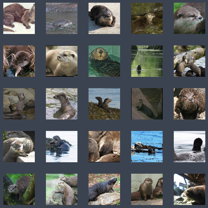
Nearest neighbor search [02:10:56]: What we can now do is we can now use nearest neighbors search. So nearest neighbors search means here is one 300 dimensional vector and here is a whole a lot of other 300 dimensional vectors, which things is it closest to? Normally that takes a very long time because you have to look through every 300 dimensional vector, calculate its distance, and find out how far away it is. But there is an amazing almost unknown library called NMSLib that does that incredibly fast. Some of you may have tried other nearest neighbor's libraries, I guarantee this is faster than what you are using — I can tell you that because it's been bench marked by people who do this stuff for a living. This is by far the fastest on every possible dimension. We want to create an index on angular distance, and we need to do it on all of our ImageNet word vectors. Adding a whole batch, create the index, and now we can query a bunch of vectors all at once, get the 10 nearest neighbors. The library uses multi-threading and is absolutely fantastic. You can install from pip (pip install nmslib) and it just works.

# use NMSLib python binding
import nmslib

def create_index(a):
    index = nmslib.init(space='angulardist')
    index.addDataPointBatch(a)
    index.createIndex()
    return index

def get_knns(index, vecs):
    return zip(*index.knnQueryBatch(vecs, k=10, num_threads=4))

def get_knn(index, vec):
    return index.knnQuery(vec, k=10)

nn_wvs = create_index(wvs)

It tells you how far away they are and their indexes [02:12:13].

idxs, dists = get_knns(nn_wvs, pred_wv)

So now we can go through and print out the top 3 so it turns out that bird actually is a limpkin. Interestingly the fourth one does not say it's a limpkin and Jeremy looked it up. He doesn't know much about birds but everything else is brown with white spots, but the 4th one isn't. So we don't know if that is actually a limpkin or if it is mislabeled but sure as heck it doesn't look like the other birds.

[ [classids[syns[id]] for id in ids[:3]]
                         for ids in idxs[start:start + 10] ]

# -----------------------------------------------------------------------------
# Output
# -----------------------------------------------------------------------------
[['mink', 'polecat', 'cougar'],
 ['badger', 'polecat', 'otter'],
 ['marmot', 'badger', 'polecat'],
 ['marmot', 'badger', 'mink'],
 ['polecat', 'badger', 'skunk'],
 ['mink', 'polecat', 'beaver'],
 ['polecat', 'cougar', 'badger'],
 ['dingo', 'wombat', 'polecat'],
 ['cockroach', 'bathtub', 'plunger'],
 ['polecat', 'skunk', 'mink']]

This is not a particularly hard thing to do because there is only a thousand ImageNet classes and it is not doing anything new. But what if we now bring in the entirety of WordNet and we now say which of those 45 thousand things is it closest to?

Search all WordNet noun classes

all_syns, all_wvs = list(zip(*syn2wv.items()))
all_wvs = np.array(all_wvs)

nn_allwvs = create_index(all_wvs)

idxs, dists = get_knns(nn_allwvs, pred_wv)

[ [classids[all_syns[id]] for id in ids[:3]] for ids in idxs[start:start + 10] ]

# -----------------------------------------------------------------------------
# Output
# -----------------------------------------------------------------------------
[['mink', 'mink', 'mink'],
 ['badger', 'polecat', 'raccoon'],
 ['marmot', 'Marmota', 'badger'],
 ['marmot', 'Marmota', 'badger'],
 ['polecat', 'Mustela', 'stoat'],
 ['mink', 'mink', 'mink'],
 ['polecat', 'Mustela', 'cougar'],
 ['dog', 'dog', 'alligator'],
 ['nosepiece', 'sweatband', 'sweatband'],
 ['polecat', 'Mustela', 'Melogale']]

Exactly the same result. It is now searching all of the WordNet.

Text -> image search [02:13:16]

Now let's do something a bit different — which is to take all of our predictions (pred_wv) so basically take our whole validation set of images and create a KNN index of the image representations because remember, it is predicting things that are meant to be word vectors. Now let's grab the fastText vector for "boat" and boat is not an ImageNet concept — yet we can now find all of the images in our predicted word vectors (i.e. our validation set) that are closest to the word boat and it works even though it is not something that was ever trained on.

def text2img(vec):
    """
    Pull images who's vector is close to our input vector (vec)
    """
    # get indices and distances
    idxs, dists = get_knn(nn_predwv, vec)
    im_res = [open_image(PATH / md.val_ds.fnames[i]) for i in idxs[:3]]
    show_imgs(im_res, 3, figsize=(9, 3))

nn_predwv = create_index(pred_wv)

en_vecd = pickle.load(open(TRANS_PATH / 'wiki.en.pkl', 'rb'))

# en_vecd is of type dict. i.e { 'sink': 300-dim word vector }
vec = en_vecd['boat'] # get the vector for boat
text2img(vec) # pull images who's vector is close to our 'boat' vector

What if we now take engine's vector and boat's vector and take their average and what if we now look in our nearest neighbors for that [02:14:04]?

vec = (en_vecd['engine'] + en_vecd['boat']) / 2
text2img(vec)

These are boats with engines. I mean, yes, the middle one is actually a boat with an engine — it just happens to have wings on as well. By the way, sail is not an ImageNet thing , neither is boat. Here is the average of two things that are not ImageNet things and yet with one exception, it's found us two sailboats.

vec = (en_vecd['sail'] + en_vecd['boat']) / 2
text2img(vec)

Image->image [02:14:35]

Okay, let's do something else crazy. Let's open up an image in the validation set. Let's call predict_array on that image to get its word vector like thing, and let's do a nearest neighbor search on all the other images.

fname = 'valid/n01440764/ILSVRC2012_val_00007197.JPEG'
img = open_image(PATH/fname)
show_img(img)

t_img = md.val_ds.transform(img)
pred = learn.predict_array(t_img[None])
idxs,dists = get_knn(nn_predwv, pred)
show_imgs([open_image(PATH / md.val_ds.fnames[i]) for i in idxs[1:4]], 3, figsize=(9, 3))

And here are all the other images of whatever that is. So you can see, this is crazy — we've trained a thing on all of ImageNet in an hour, using a custom head that required basically like two lines of code, and these things run in 300 milliseconds to do these searches.

Jeremy taught this basic idea last year as well, but it was in Keras, and it was pages and pages of code, and everything took a long time and complicated. And back then, Jeremy said he can't begin to think all of the stuff you could do with this. He doesn't think anybody has really thought deeply about this yet, but he thinks it's fascinating. So go back and read the DeViSE paper because Andrea had a whole bunch of other thoughts and now that it is so easy to do, hopefully people will dig into this now. Jeremy thinks it's crazy and amazing.