Lesson 3 - Multi-label, Segmentation, Image Regression, and More

These are my personal notes from fast.ai Live (the new International Fellowship programme) course and will continue to be updated and improved if I find anything useful and relevant while I continue to review the course to study much more in-depth. Thanks for reading and happy learning!

Live date: 9 Nov 2018, GMT+8

Topics

Multi-label classification
Kaggle Planet Amazon dataset of satellite images
fastai Data Block API
fastai DataBunch class
Image segmentation with CamVid
U-Net
Learning rate annealing
Mixed precision training
Image regression with BIWI head pose dataset
NLP classification
Universal approximation theorem

Lesson Resources

Assignments

Run lesson 3 notebooks.
Replicate lesson 3 notebooks with your own dataset.
Dig into the Data Block API.

Other Resources

Blog Posts and Articles

Universal Language Model Fine-tuning (ULMFiT) for Text Classification used in language_model_learner
Michael Nielsen's book
Quick and easy model deployment on Zeit Now guide
Data Block API

Other Useful Information

Useful online courses for machine learning background:
- Machine Learning taught by Andrew Ng (Coursera)
- Introduction to Machine Learning for Coders taught by Jeremy Howard
Python partials
Nov 14 Meetup - Conversation between Jeremy Howard and Leslie Smith
List of vision transforms

Useful Tools and Libraries

Fast.ai Video Viewer with searchable transcript
MoviePy Python module for video editing mentioned by Rachel
WebRTC example for web video from Ethan Sutin

Papers

Optional reading
- Cyclical Learning Rates for Training Neural Networks by Leslie Smith

My Notes

A quick correction on citation.

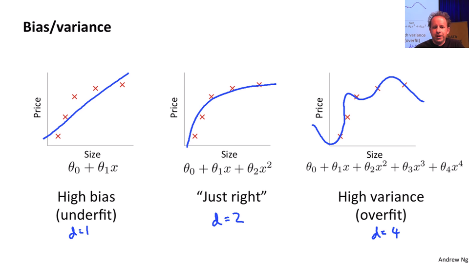
This chart originally cane from Andrew Ng's excellent machine learning course on Coursera. Apologies for the incorrect citation.

Machine Learning course

Andrew Ng's machine learning course on Coursera is great. In some ways, it's a little dated but a lot of the content is as appropriate as ever and taught in a bottom-up style. So it can be quite nice to combine it with our top down style and meet somewhere in the middle.

Also, if you are interested in machine learning foundations, you should check out our machine learning course as well. It is about twice as long as this deep learning course and takes you much more gradually through some of the foundational stuff around validation sets, model interpretation, how PyTorch tensor works, etc. I think all these courses together, if you really dig deeply into the material, do all of them. I know a lot of people who have and end up saying "oh, I got more out of each one by doing a whole lot". Or you can backwards and forwards to see which one works for you.

Deploy web app with your model in production

We started talking about deploying your web app last week. One thing that's going to make life a lot easier for you is that https://course-v3.fast.ai/ has a production section where right now we have one platform but more will be added showing you how to deploy your web app really easily. When I say easily, for example, here is how to deploy on Zeit guide created by San Francisco study group member, Navjot.

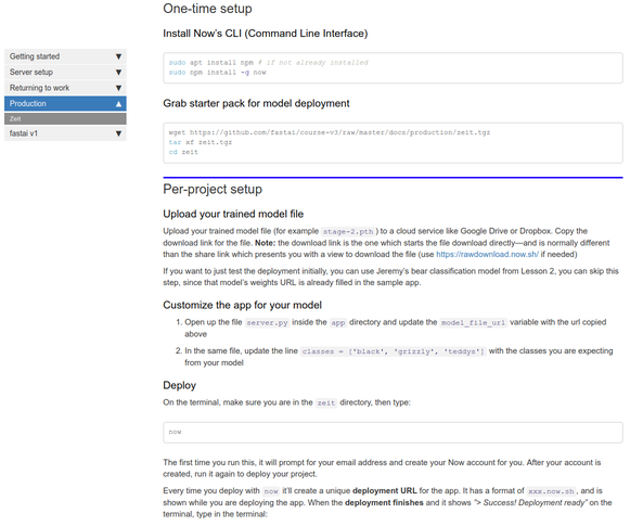
As you can see, it's just a page. There's almost nothing to and it's free. It's not going to serve 10,000 simultaneous requests but it'll certainly get you started and I found it works really well. It's fast. Deploying a model doesn't have to be slow or complicated anymore. And the nice thing is, you can use this for a Minimum Viable Product (MVP) if you do find it's starting to get a thousand simultaneous requests, then you know that things are working out and you can start to upgrade your instance types or add to a more traditional big engineering approach. If you actually use this starter kit, it will create my teddy bear finder for you. So the idea is, this template is as simple as possible. So you can fill in your own style sheets, your own custom logic, and so forth. This is designed to be a minimal thing, so you can see exactly what's going on. The backend is a simple REST style interface that sends back JSON and the frontend is a super simple little JavaScript thing. It should be a good way to get a sense of how to build a web app which talks to a PyTorch model.

Examples of web apps people have built during the week 3:36

Edward Ross built the "What Australian car is that?" app.

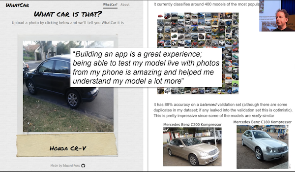
I thought it was interesting that Edward said on the forum that building of this app was actually a great experience in terms of understanding how the model works himself better. It's interesting that he's describing trying it out on his phone. A lot of people think "oh, if I want something on my phone, I have to create some kind of mobile TensorFlow, ONNX, whatever tricky mobile app"﹣you really don't. You can run it all in the Cloud and make it just a web app or use some kind of simple little GUI frontend that talks to a REST backend. It's not that often that you'll need to actually run stuff on the phone. So this is a good example of that.


Guitar Classifier by Christian Werner	Healthy or Not! by Nikhil Utane
Hummingbird Classifier by Nissan Dookeran	Edible Mushroom? by Ramon
Cousin Recognizer by Charlie Harrington	Emotion Classifier by Ethan Sutin and Team 26
American Sign Language by Keyur Paralkar	Your City from Space by Henri Palacci
Univariate time series as images using Gramian Angular Field by Ignacio Oguiza	Face Expression Recognition by Pierre Guillou
Tumor-normal sequencing by Alena Harley

Nice to see what people have been building in terms of both web apps and just classifiers. What we are going to do today is look at a whole a lot more different types of model that you can build and we're going to zip through them pretty quickly and then we are going to go back and see how all these things work and what the common denominator is. All of these things, you can create web apps from these as well but you'll have to think about how to slightly change that template to make it work with these different applications. I think that'll be a really good exercise in making sure you understand the material.

Multi-label classification with Planet Amazon dataset [9:51]

lesson3-planet.ipynb

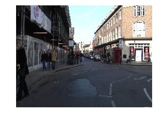
The first one we're going to look at is a dataset of satellite images. Satellite imaging is a really fertile area for deep learning. Certainly a lot of people are already using deep learning in satellite imaging but only scratching the surface. The dataset we are going to look at looks like this:

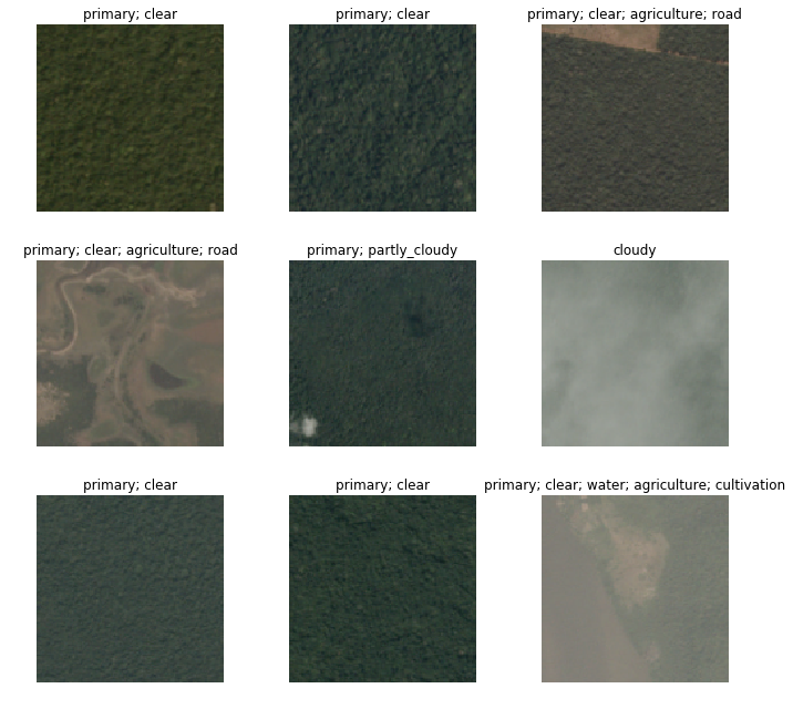
It has satellite tiles and for each one, as you can see, there's a number of different labels for each tile. One of the labels always represents the weather (e.g. cloudy, partly_cloudy). And all of the other labels tell you any interesting features that are seen there. So primary means primary rainforest, agriculture means there's some farming, road means road, and so forth. As I am sure you can tell, this is a little different to all the classifiers we've seen so far because there's not just one label, there's potentially multiple labels. So multi-label classification can be done in a very similar way but the first thing we are going to need to do is to download the data.

Downloading the data [11:02]

This data comes from Kaggle. Kaggle is mainly known for being a competitions website and it's really great to download data from Kaggle when you're learning because you can see how would I have gone in that competition. And it's a good way to see whether you know what you are doing. I tend to think the goal is to try and get in the top 10%. In my experience, all the people in the top 10% of a competition really know what they're doing. So if you can get in the top 10%, then that's a really good sign.

Pretty much every Kaggle dataset is not available for download outside of Kaggle (at least competition datasets) so you have to download it through Kaggle. The good news is that Kaggle provides a python-based downloader tool which you can use, so we've got a quick description here of how to download stuff from Kaggle.

You first have to install the Kaggle download tool via pip.

#! pip install kaggle --upgrade

What we tend to do when there's one-off things to do is we show you the commented out version in the notebook and you can just remove the comment. If you select a few lines and then hit ctrl+/, it uncomment them all. Then when you are done, select them again, ctrl+/ again and re-comments them all. So this line will install kaggle for you. Depending on your platform, you may need sudo or /something/pip, you may need source activate so have a look on the setup instructions instructions or the returning to work instructions on the course website to see when we do conda install, you have to the same basic steps for your pip install.

Once you've got that module installed, you can then go ahead and download the data. Basically it's as simple as saying kaggle competitions download -c competition_name -f file_name the only other steps you do that is you have to authenticate yourself and there is a little bit of information here on exactly how you can go about downloading from Kaggle the file containing your API authentication information. I wouldn't bother going through it here, but just follow these steps.

Then you need to upload your credentials from Kaggle on your instance. Login to kaggle and click on your profile picture on the top left corner, then 'My account'. Scroll down until you find a button named 'Create New API Token' and click on it. This will trigger the download of a file named 'kaggle.json'.

Upload this file to the directory this notebook is running in, by clicking "Upload" on your main Jupyter page, then uncomment and execute the next two commands (or run them in a terminal).

#! mkdir -p ~/.kaggle/
#! mv kaggle.json ~/.kaggle/

You're all set to download the data from Planet competition. You first need to go to its main page and accept its rules, and run the two cells below (uncomment the shell commands to download and unzip the data). If you get a 403 forbidden error it means you haven't accepted the competition rules yet (you have to go to the competition page, click on Rules tab, and then scroll to the bottom to find the accept button).

path = Config.data_path()/'planet'
path.mkdir(exist_ok=True)
path

PosixPath('/home/jhoward/.fastai/data/planet')

# ! kaggle competitions download -c planet-understanding-the-amazon-from-space -f train-jpg.tar.7z -p {path}
# ! kaggle competitions download -c planet-understanding-the-amazon-from-space -f train_v2.csv -p {path}
# ! unzip -q -n {path}/train_v2.csv.zip -d {path}

Sometimes stuff on Kaggle is not just zipped or tared but it's compressed with a program called 7zip which will have a .7z extension. If that's the case, you'll need to either apt install p7zip or here is something really nice. Some kind person has created a conda installation of 7zip that works on every platform. So you can always just run this conda install ﹣doesn't even require a sudo or anything like that. This is actually a good example of where conda is super handy. You can actually install binaries and libraries and stuff like that and it's nicely cross-platform. So if you don't have 7zip installed, that's a good way to get it.

To extract the content of this file, we'll need 7zip, so uncomment the following line if you need to install it (or run sudo apt install p7zip in your terminal).

# ! conda install -y -c haasad eidl7zip

This is how you unzip a 7zip file. In this case, it's tared and 7zipped, so you can do this all in one step. 7za is the name of the 7zip archival program you would run.

That's all basic stuff which if you are not familiar with the command line and stuff, it might take you a little bit of experimenting to get it working. Feel free to ask on the forum, make sure you search the forum first to get started.

# ! 7za -bd -y -so x {path}/train-jpg.tar.7z | tar xf - -C {path}

Multiclassification [14:49]

Once you've got the data downloaded and unzipped, you can take a look at it. In this case, because we have multiple labels for each tile, we clearly can't have a different folder for each image telling us what the label is. We need some different way to label it. The way Kaggle did it was they provided a CSV file that had each file name along with a list of all the labels. So in order to just take a look at that CSV file, we can read it using the Pandas library. If you haven't used pandas before, it's kind of the standard way of dealing with tabular data in Python. It pretty much always appears in the pd namespace. In this case we're not really doing anything with it other than just showing you the contents of this file. So we can read it, take a look at the first few lines, and there it is:

df = pd.read_csv(path/'train_v2.csv')
df.head()

	image_name	tags
0	train_0	haze primary
1	train_1	agriculture clear primary water
2	train_2	clear primary
3	train_3	clear primary
4	train_4	agriculture clear habitation primary road

We want to turn this into something we can use for modeling. So the kind of object that we use for modeling is an object of the DataBunch class. We have to somehow create a data bunch out of this. Once we have a data bunch, we'll be able to go .show_batch to take a look at it. And then we'll be able to go create_cnn with it, and we would be able to start training.

So really the trickiest step previously in deep learning has often been getting your data into a form that you can get it into a model. So far we've been showing you how to do that using various "factory methods" which are methods where you say "I want to create this kind of data from this kind of source with these kinds of options." That works fine, sometimes, and we showed you a few ways of doing it over the last couple of weeks. But sometimes you want more flexibility, because there's so many choices that you have to make about:

Where do the files live
What's the structure they're in
How do the labels appear
How do you spit out the validation set
How do you transform it

Data Block API [17:05]

So we've got this unique API that I'm really proud of called the Data Block API. The Data Block API makes each one of those decisions a separate decision that you make. There are separate methods with their own parameters for every choice that you make around how to create/set up my data.

Announcement: 📢 2018-11-13: there's been one change to fastai v1.0.24 and above—ImageFileList is now called ImageItemList. You'll need to make that change in any notebooks that you've created too. Reference: forum: Name 'ImageFileList' is not defined in fastai version 1.0.24

tfms = get_transforms(flip_vert=True, max_lighting=0.1, max_zoom=1.05, max_warp=0.)

np.random.seed(42)
src = (ImageItemList.from_folder(path)
       .label_from_csv('train_v2.csv',sep=' ',folder='train-jpg',suffix='.jpg')
       .random_split_by_pct(0.2))

data = (src.datasets()
        .transform(tfms, size=128)
        .databunch().normalize(imagenet_stats))

For example, to grab the planet data we would say:

We've got a list of image files that are in a folder
They're labeled based on a CSV with this name (train_v2.csv)
- They have this separator ( ) ﹣remember I showed you back here that there's a space between them. By passing in separator, it's going to create multiple labels.
- The images are in this folder (train-jpg)
- They have this suffix (.jpg)
They're going to randomly spit out a validation set with 20% of the data
We're going to create datasets from that, which we are then going to transform with these transformations (tfms)
Then we going to create a data bunch out of that, which we will then normalize using these statistics (imagenet_stats)

So there's all these different steps. To give you a sense of what that looks like, the first thing I'm going to do is go back and explain what are all of the PyTorch and fastai classes you need to know about that are going to appear in this process. Because you're going to see them all the time in the fastai docs and PyTorch docs.

Dataset (PyTorch) [18:30]

The first one you need to know about is a class called a Dataset. The Dataset class is part of PyTorch and this is the source code for the Dataset class:

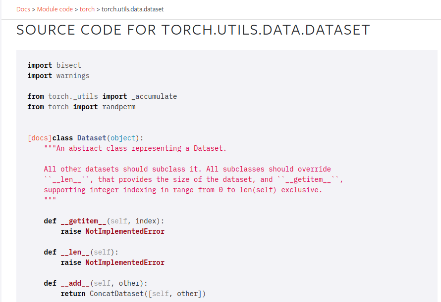
As you can see. it actually does nothing at all. The Dataset class in PyTorch defines two things: __getitem__ and __len__. In Python these special things that are "underscore underscore something underscore underscore" ﹣Pythonists call them "dunder" something. So these would be "dunder get items" and "dunder len". They're basically special magical methods with some special behavior. This particular method means that your object, if you had an object called o, it can be indexed with square brackets (e.g. o[3]). So that would call __getitem__ with 3 as the index.

Then this one called __len__ means that you can go len(o) and it will call that method. In this case, they're both not implemented. That is to say, although PyTorch says "in order to tell PyTorch about your data, you have to create a dataset", it doesn't really do anything to help you create the dataset. It just defines what the dataset needs to do. In other words, the starting point for your data is something where you can say:

What is the third item of data in my dataset (that's what __getitem__ does)
How big is my dataset (that's what __len__ does)

Fastai has lots of Dataset subclasses that do that for all different kinds of stuff. So far, you've been seeing image classification datasets. They are datasets where __getitem__ will return an image and a single label of what is that image. So that's what a dataset is.

DataLoader (PyTorch) [20:37]

Now a dataset is not enough to train a model. The first thing we know we have to do, if you think back to the gradient descent tutorial last week is we have to have a few images/items at a time so that our GPU can work in parallel. Remember we do this thing called a "mini-batch"? Mini-batch is a few items that we present to the model at a time that it can train from in parallel. To create a mini-batch, we use another PyTorch class called a DataLoader.

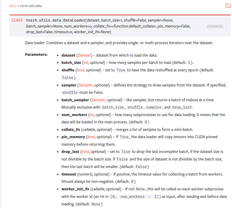
A DataLoader takes a dataset in its constructor, so it's now saying "oh this is something I can get the third item and the fifth item and the ninth item." It's going to:

Grab items at random
Create a batch of whatever size you asked for
Pop it on the GPU
Send it off to your model for you

So a DataLoader is something that grabs individual items, combines them into a mini-batch, pops them on the GPU for modeling. So that's called a DataLoader and that comes from a Dataset.

You can see, already there are choices you have to make: what kind of dataset am I creating, what is the data for it, where it's going to come from. Then when I create my DataLoader: what batch size do I want to use.

DataBunch (fastai) [21:59]

It still isn't enough to train a model, because we've got no way to validate the model. If all we have is a training set, then we have no way to know how we're doing because we need a separate set of held out data, a validation set, to see how we're getting along.

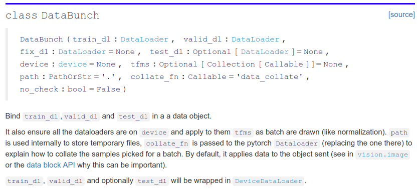
For that we use a fastai class called a DataBunch. A DataBunch is something which binds together a training data loader (train_dl) and a valid data loader (valid_dl). When you look at the fastai docs when you see these mono spaced font things, they're always referring to some symbol you can look up elsewhere. In this case you can see train_dl is the first argument of DataBunch. There's no point knowing that there's an argument with a certain name unless you know what that argument is, so you should always look after the : to find out that is a DataLoader. So when you create a DataBunch, you're basically giving it a training set data loader and a validation set data loader. And that's now an object that you can send off to a learner and start fitting.

They're the basic pieces. Coming back to here, these are all the stuff which is creating the dataset:

With the dataset, the indexer returns two things: the image and the labels (assuming it's an image dataset).

where do the images come from
where do the labels come from
then I'm going to create two separate data sets the training and the validation
.datasets() actually turns them into PyTorch datasets
.transform() is the thing that transforms them
.databunch() is actually going to create the the DataLoader and the DataBunch in one go

Data Block API examples [23:56]

Let's look at some examples of this Data Block API because once you understand the Data Block API, you'll never be lost for how to convert your dataset into something you can start modeling with.

data_block.ipynb

MNIST

Here are some examples of using the Data Block API. For example, if you're looking at MNIST (the pictures and classes of handwritten numerals), you can do something like this:

path = untar_data(URLs.MNIST_TINY)
tfms = get_transforms(do_flip=False)
path.ls()

[PosixPath('/home/jhoward/.fastai/data/mnist_tiny/valid'),
 PosixPath('/home/jhoward/.fastai/data/mnist_tiny/models'),
 PosixPath('/home/jhoward/.fastai/data/mnist_tiny/train'),
 PosixPath('/home/jhoward/.fastai/data/mnist_tiny/test'),
 PosixPath('/home/jhoward/.fastai/data/mnist_tiny/labels.csv')]

(path/'train').ls()

[PosixPath('/home/jhoward/.fastai/data/mnist_tiny/train/3'),
 PosixPath('/home/jhoward/.fastai/data/mnist_tiny/train/7')]

data = (ImageItemList.from_folder(path)  #Where to find the data? -> in path and its subfolders
        .label_from_folder()             #How to label? -> depending on the folder of the filenames
        .split_by_folder()               #How to split in train/valid? -> use the folders
        .add_test_folder()               #Optionally add a test set
        .datasets()                      #How to convert to datasets?
        .transform(tfms, size=224)       #Data augmentation? -> use tfms with a size of 224
        .databunch())                    #Finally? -> use the defaults for conversion to ImageDataBunch

What kind of data set is this going to be?
- It's going to come from a list of image files which are in some folder.
- They're labeled according to the folder name that they're in.
- We're going to split it into train and validation according to the folder that they're in (train and valid).
- You can optionally add a test set. We're going to be talking more about test sets later in the course.
- We'll convert those into PyTorch datasets now that that's all set up.
- We will then transform them using this set of transforms (tfms), and we're going to transform into something of this size (224).
- Then we're going to convert them into a data bunch.

So each of those stages inside these parentheses are various parameters you can pass to customize how that all works. But in the case of something like this MNIST dataset, all the defaults pretty much work, so this is all fine.

data.train_ds[0]

(Image (3, 224, 224), 0)

Here it is. data.train_ds is the dataset (not the data loader) so I can actually index into it with a particular number. So here is the zero indexed item in the training data set: it's got an image and a label.

data.show_batch(rows=3, figsize=(5,5))

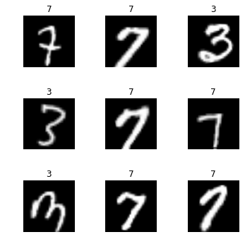
We can show batch to see an example of the pictures of it. And we could then start training.

data.valid_ds.classes

['3', '7']

Here are the classes that are in that dataset. This little cut-down sample of MNIST has 3's and 7's.

Planet [26:01]

Here's an example using Planet dataset. This is actually again a little subset of planet we use to make it easy to try things out.

planet = untar_data(URLs.PLANET_TINY)
planet_tfms = get_transforms(flip_vert=True, max_lighting=0.1, max_zoom=1.05, max_warp=0.)
data = ImageDataBunch.from_csv(planet, folder='train', size=128, suffix='.jpg', sep = ' ', ds_tfms=planet_tfms)

With the Data Block API we can rewrite this like that:

data = (ImageItemList.from_folder(planet)
        #Where to find the data? -> in planet and its subfolders
        .label_from_csv('labels.csv', sep=' ', folder='train', suffix='.jpg')
        #How to label? -> use the csv file labels.csv in path,
        #add .jpg to the names and take them in the folder train
        .random_split_by_pct()
        #How to split in train/valid? -> randomly with the default 20% in valid
        .datasets()
        #How to convert to datasets? -> use ImageMultiDataset
        .transform(planet_tfms, size=128)
        #Data augmentation? -> use tfms with a size of 128
        .databunch())
        #Finally? -> use the defaults for conversion to databunch

In this case:

Again, it's an ImageItemList
We are grabbing it from a folder
This time we're labeling it based on a CSV file
We're randomly splitting it (by default it's 20%)
Creating data sets
Transforming it using these transforms (planet_tfms), we're going to use a smaller size (128).
Then create a data bunch

data.show_batch(rows=3, figsize=(10,8))

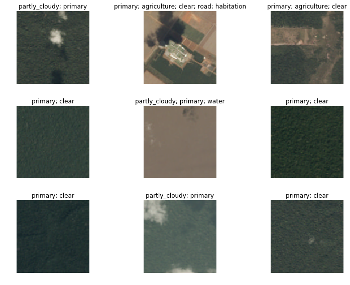
There it is. Data bunches know how to draw themselves amongst other things.

CamVid [26:38]

Here's some more examples we're going to be seeing later today.

camvid = untar_data(URLs.CAMVID_TINY)
path_lbl = camvid/'labels'
path_img = camvid/'images'

codes = np.loadtxt(camvid/'codes.txt', dtype=str); codes

array(['Animal', 'Archway', 'Bicyclist', 'Bridge', 'Building', 'Car', 'CartLuggagePram', 'Child', 'Column_Pole',
       'Fence', 'LaneMkgsDriv', 'LaneMkgsNonDriv', 'Misc_Text', 'MotorcycleScooter', 'OtherMoving', 'ParkingBlock',
       'Pedestrian', 'Road', 'RoadShoulder', 'Sidewalk', 'SignSymbol', 'Sky', 'SUVPickupTruck', 'TrafficCone',
       'TrafficLight', 'Train', 'Tree', 'Truck_Bus', 'Tunnel', 'VegetationMisc', 'Void', 'Wall'], dtype='<U17')

get_y_fn = lambda x: path_lbl/f'{x.stem}_P{x.suffix}'

x.stem is Python pathlib pure path method. Pure path objects provide path-handling operations which don’t actually access a filesystem.

data = (ImageItemList.from_folder(path_img)                #Where are the input files? -> in path_img
        .label_from_func(get_y_fn)                         #How to label? -> use get_y_fn
        .random_split_by_pct()                             #How to split between train and valid? -> randomly
        .datasets(SegmentationDataset, classes=codes)      #How to create a dataset? -> use SegmentationDataset
        .transform(get_transforms(), size=96, tfm_y=True)  #Data aug -> Use standard tfms with tfm_y=True
        .databunch(bs=64))                                 #Lastly convert in a databunch.

data.show_batch(rows=2, figsize=(5,5))

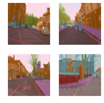
What if we look at this data set called CAMBID? CAMVID looks like this. It contains pictures and every pixel in the picture is color coded. So in this case:

We have a list of files in a folder
We're going to label them using a function. So this function (get_y_fn) is basically the thing which tells it whereabouts of the color coding for each pixel. It's in a different place.
Randomly split it in some way
Create some datasets in some way. We can tell it for our particular list of classes, how do we know what pixel you know value 1 versus pixel value 2 is. That was something that we can read in.
Some transforms
Create a data bunch. You can optionally pass in things like what batch size do you want.

Again, it knows how to draw itself and you can start learning with that.

COCO [27:41]

One more example. What if we wanted to create something like this:

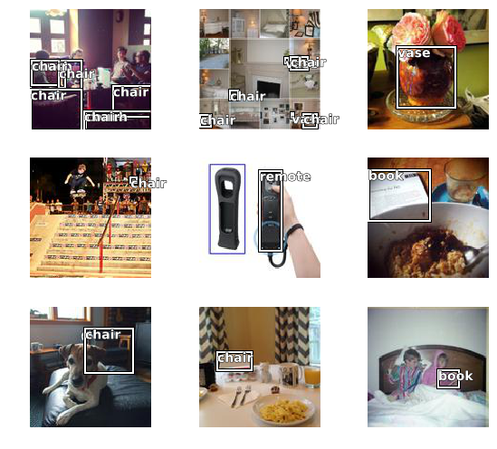
This is called an object detection dataset. Again, we've got a little minimal COCO dataset. COCO is the most famous academic dataset for object detection.

coco = untar_data(URLs.COCO_TINY)
images, lbl_bbox = get_annotations(coco/'train.json')
img2bbox = {img:bb for img, bb in zip(images, lbl_bbox)}
get_y_func = lambda o:img2bbox[o.name]

data = (ImageItemList.from_folder(coco)
        #Where are the images? -> in coco
        .label_from_func(get_y_func)
        #How to find the labels? -> use get_y_func
        .random_split_by_pct()
        #How to split in train/valid? -> randomly with the default 20% in valid
        .datasets(ObjectDetectDataset)
        #How to create datasets? -> with ObjectDetectDataset
        #Data augmentation? -> Standard transforms with tfm_y=True
        .databunch(bs=16, collate_fn=bb_pad_collate))
        #Finally we convert to a DataBunch and we use bb_pad_collate

We can create it using the same process:

Grab a list of files from a folder.
Label them according to this little function (get_y_func).
Randomly split them.
Create an object detection dataset.
Create a data bunch. In this case you have to use generally smaller batch sizes or you'll run out of memory. And you have to use something called a "collation function".

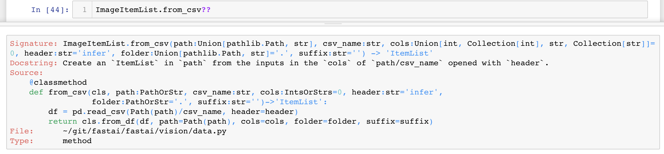
Once that's all done we can again show it and here is our object detection data set. So you get the idea. So here's a really convenient notebook. Where will you find this? Ah, this notebook is the documentation. Remember how I told you that all of the documentation comes from notebooks? You'll find them in fastai repo in docs_src. This which you can play with and experiment with inputs and outputs, and try all the different parameters, you will find the Data Block API examples of use, if you go to the documentation here it is - the Data Block API examples of use.

Everything that you want to use in fastai, you can look it up in the documentation. There is also search functionality available:

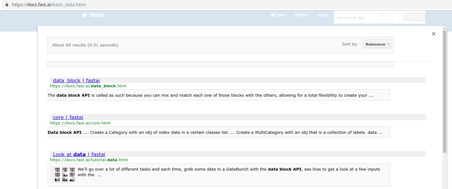
So once you find some documentation that you actually want to try playing with yourself, just look up the name (e.g. data_block.html) and then you can open up a notebook with the same name (e.g. data_block.ipynb) in the fastai repo and play with it yourself.

Creating satellite image DataBunch [29:35]

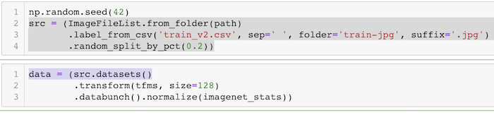
That was a quick overview of this really nice Data Block API, and there's lots of documentation for all of the different ways you can label inputs, split data, and create datasets. So that's what we're using for Planet.

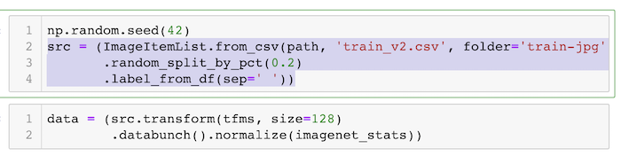
In the documentation, these two steps were all joined up together:

np.random.seed(42)
src = (ImageItemList.from_folder(path)
       .label_from_csv('train_v2.csv', sep=' ', folder='train-jpg', suffix='.jpg')
       .random_split_by_pct(0.2))

data = (src.datasets()
        .transform(tfms, size=128)
        .databunch().normalize(imagenet_stats))

We can certainly do that here too, but you'll learn in a moment why it is that we're actually splitting these up into two separate steps which is also fine as well.

A few interesting points about this.

Transforms: transforms by default will flip randomly each image, but they'll actually randomly only flip them horizontally. If you're trying to tell if something is a cat or a dog, it doesn't matter whether it's pointing left or right. But you wouldn't expect it to be upside down On the other hand satellite imagery whether something's cloudy or hazy or whether there's a road there or not could absolutely be flipped upside down. There's no such thing as a right way up from space. So flip_vert which defaults to False, we're going to flip over to True to say you should actually do that. And it doesn't just flip it vertically, it actually tries each possible 90-degree rotation (i.e. there are 8 possible symmetries that it tries out).
Warp: perspective warping is something which very few libraries provide, and those that do provide it it tends to be really slow. I think fastai is the first one to provide really fast perspective warping. Basically, the reason this is interesting is if I look at you from below versus above, your shape changes. So when you're taking a photo of a cat or a dog, sometimes you'll be higher, sometimes you'll be lower, then that kind of change of shape is certainly something that you would want to include as you're creating your training batches. You want to modify it a little bit each time. Not true for satellite images. A satellite always points straight down at the planet. So if you added perspective warping, you would be making changes that aren't going to be there in real life. So I turn that off.

This is all something called data augmentation. We'll be talking a lot more about it later in the course. But you can start to get a feel for the kinds of things that you can do to augment your data. In general, maybe the most important one is if you're looking at astronomical data, pathology digital slide data, or satellite data where there isn't really an up or down, turning on flip verticals true is generally going to make your models generalize better.

Creating multi-label classifier [35:59]

Now to create a multi-label classifier that's going to figure out for each satellite tile what's the weather and what else what can I see in it, there's basically nothing else to learn. Everything else that you've already learned is going to be exactly nearly the same.

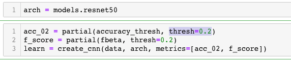
arch = models.resnet50

acc_02 = partial(accuracy_thresh, thresh=0.2)
f_score = partial(fbeta, thresh=0.2)
learn = create_cnn(data, arch, metrics=[acc_02, f_score])

When I first built built this notebook, I used resnet34 as per usual. Then I tried resnet50 as I always like to do. I found resnet50 helped a little bit and I had some time to run it, so in this case I was using resnet50.

There's one more change I make which is metrics. To remind you, a metric has got nothing to do with how the model trains. Changing your metrics will not change your resulting model at all. The only thing that we use metrics for is we print them out during training.

lr = 0.01

learn.fit_one_cycle(5, slice(lr))

Total time: 04:17
epoch  train_loss  valid_loss  accuracy_thresh  fbeta
    0.115247    0.103319    0.950703         0.910291  (00:52)
    0.108289    0.099074    0.953239         0.911656  (00:50)
    0.102342    0.092710    0.953348         0.917987  (00:51)
    0.095571    0.085736    0.957258         0.926540  (00:51)
    0.091275    0.085441    0.958006         0.926234  (00:51)

Here it's printing out accuracy and this other metric called fbeta. If you're trying to figure out how to do a better job with your model, changing the metrics will never be something that you need to do. They're just to show you how you're going.

You can have one metric, no metrics, or a list of multiple metrics to be printed out as your models training. In this case, I want to know two things:

The accuracy
How would I go on Kaggle

Kaggle told me that I'm going to be judged on a particular metric called the F score. I'm not going to bother telling you about the F score﹣it's not really interesting enough to be worth spending your time on. But it's basically this. When you have a classifier, you're going to have some false positives and some false negatives. How do you weigh up those two things to create a single number? There's lots of different ways of doing that and something called the F score is a nice way of combining that into a single number. And there are various kinds of F scores: F1, F2 and so forth. And Kaggle said in the competition rules, we're going to use a metric called F2.

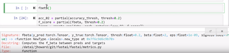
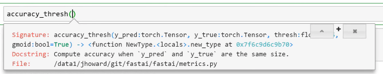
We have a metric called fbeta. In other words, it's F with 1, 2, or whatever depending on the value of beta. We can have a look at its signature and it has a threshold and a beta. The beta is 2 by default, and Kaggle said that they're going to use F 2 so I don't have to change that. But there's one other thing that I need to set which is a threshold.

What does that mean? Here's the thing. Do you remember we had a little look the other day at the source code for the accuracy metric? And we found that it used this thing called argmax. The reason for that was we had this input image that came in, it went through our model, and at the end it came out with a table of ten numbers. This is if we're doing MNIST digit recognition and the ten numbers were the probability of each of the possible digits. Then we had to look through all of those and find out which one was the biggest. So the function in Numpy, PyTorch, or just math notation that finds the biggest in returns its index is called argmax.

To get the accuracy for our pet detector, we use this accuracy function the called argmax to find out which class ID pet was the one that we're looking at. Then it compared that to the actual, and then took the average. That was the accuracy.

[37:23]

We can't do that for satellite recognition because there isn't one label we're looking for﹣there's lots. A data bunch has a special attribute called c and c is going to be how many outputs do we want our model to create. For any kind of classifier, we want one probability for each possible class. In other words, data.c for classifiers is always going to be equal to the length of data.classes.

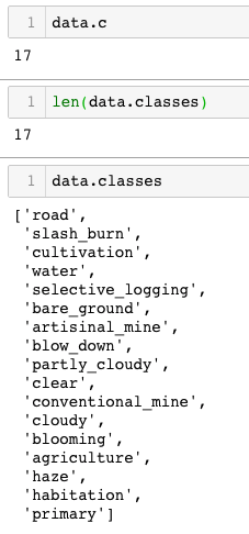
They are the 17 possibilities. So we're going to have one probability for each of those. But then we're not just going to pick out one of those 17, we're going to pick out n of those 17. So what we do is, we compare each probability to some threshold. Then we say anything that's higher than that threshold, we're going to assume that the models saying it does have that feature. So we can pick that threshold.

I found that for this particular dataset, a threshold of 0.2 seems to generally work pretty well. This is the kind of thing you can easily just experiment to find a good threshold. So I decided I want to print out the accuracy at a threshold of 0.2.

The normal accuracy function doesn't work that way. It doesn't argmax. We have to use a different accuracy function called accuracy_thresh. That's the one that's going to compare every probability to a threshold and return all the things higher than that threshold and compare accuracy that way.

Python 3 `partial` [39:17]

One of the things we had passed in is thresh. Now of course our metric is going to be calling our function for us, so we don't get to tell it every time it calls back what threshold do we want, so we really want to create a special version of this function that always uses a threshold of 0.2. One way to do that would be defining a function acc_02 as below:

def acc_02(inp, targ): return accuracy_thresh(inp, targ, thresh=0.2)

We could do it that way. But it's so common that computer science has a term for that it's called a "partial" / "partial function application" (i.e. create a new function that's just like that other function but we are always going to call it with a particular parameter).

Python 3 has something called partial that takes some function and some list of keywords and values, and creates a new function that is exactly the same as this function (accurasy_thresh) but is always going to call it with that keyword argument (thresh=0.2).

acc_02 = partial(accuracy_thresh, thresh=0.2)

This is a really common thing to do particularly with the fastai library because there's lots of places where you have to pass in functions and you very often want to pass in a slightly customized version of a function so here's how you do it.

Similarly, fbeta with thresh=0.2:

acc_02 = partial(accuracy_thresh, thresh=0.2)
f_score = partial(fbeta, thresh=0.2)
learn = create_cnn(data, arch, metrics=[acc_02, f_score])

I can pass them both in as metrics and I can then go ahead and do all the normal stuff.

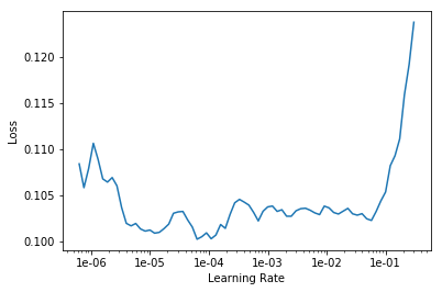
learn.lr_find()

learn.recorder.plot()

Find the thing with the steepest slope—so somewhere around 1e-2, make that our learning rate.

lr = 0.01

Then fit for awhile with 5, slice(lr) and see how we go.

learn.fit_one_cycle(5, slice(lr))

Total time: 04:17
epoch  train_loss  valid_loss  accuracy_thresh  fbeta
    0.115247    0.103319    0.950703         0.910291  (00:52)
    0.108289    0.099074    0.953239         0.911656  (00:50)
    0.102342    0.092710    0.953348         0.917987  (00:51)
    0.095571    0.085736    0.957258         0.926540  (00:51)
    0.091275    0.085441    0.958006         0.926234  (00:51)

So we've got an accuracy of about 96% and F beta of about 0.926 and so you could then go and have a look at Planet private leaderboard. The top 50th is about 0.93 so we kind of say like oh we're on the right track. So as you can see, once you get to a point that the data is there, there's very little extra to do most of the time.

Question: When your model makes an incorrect prediction in a deployed app, is there a good way to “record” that error and use that learning to improve the model in a more targeted way? [42:01]

That's a great question. The first bit﹣is there a way to record that? Of course there is. You record it. That's up to you. Maybe some of you can try it this week. You need to have your user tell you that you were wrong. This Australian car you said it was a Holden and actually it's a Falcon. So first of all. you'll need to collect that feedback and the only way to do that is to ask the user to tell you when it's wrong. So you now need to record in some log somewhere﹣something saying you know this was the file, I've stored it here, this was the prediction I made, this was the actual that they told me. Then at the end of the day or at the end of the week, you could set up a little job to run something or you can manually run something. What are you going to do? You're going to do some fine-tuning. What does fine-tuning look like? Good segue Rachel! It looks like this.

So let's pretend here's your saved model:

learn.save('stage-1-rn50')

Then we unfreeze:

learn.unfreeze()

learn.lr_find()
learn.recorder.plot()

Then we fit a little bit more. Now in this case, I'm fitting with my original dataset. But you could create a new data bunch with just the misclassified instances and go ahead and fit. The misclassified ones are likely to be particularly interesting. So you might want to fit at a slightly higher learning rate to make them really mean more or you might want to run them through a few more epochs. But it's exactly the same thing. You just call fit with your misclassified examples and passing in the correct classification. That should really help your model quite a lot.

There are various other tweaks you can do to this but that's the basic idea.

learn.fit_one_cycle(5, slice(1e-5, lr/5))

Total time: 05:48
epoch  train_loss  valid_loss  accuracy_thresh  fbeta
    0.096917    0.089857    0.964909         0.923028  (01:09)
    0.095722    0.087677    0.966341         0.924712  (01:09)
    0.088859    0.085950    0.966813         0.926390  (01:09)
    0.085320    0.083416    0.967663         0.927521  (01:09)
    0.081530    0.082129    0.968121         0.928895  (01:09)

learn.save('stage-2-rn50')

Question: Could someone talk a bit more about the Data Block ideology? I'm not quite sure how the blocks are meant to be used. Do they have to be in a certain order? Is there any other library that uses this type of programming that I could look at? [44:01]

Yes, they do have to be in a certain order and it's basically the order that you see in the example of use.

data = (ImageItemList.from_folder(path) #Where to find the data? -> in path and its subfolders
        .split_by_folder()              #How to split in train/valid? -> use the folders
        .label_from_folder()            #How to label? -> depending on the folder of the filenames
        .add_test_folder()              #Optionally add a test set (here default name is test)
        .transform(tfms, size=64)       #Data augmentation? -> use tfms with a size of 64
        .databunch())                   #Finally? -> use the defaults for conversion to ImageDataBunch

What kind of data do you have?
Where does it come from?
How do you split it?
How do you label it?
What kind of datasets do you want?
Optionally, how do I transform it?
How do I create a data bunch from?

They're the steps. We invented this API. I don't know if other people have independently invented it. The basic idea of a pipeline of things that dot into each other is pretty common in a number of places﹣not so much in Python, but you see it more in JavaScript. Although this kind of approach of each stage produces something slightly different, you tend to see it more in like ETL software (extraction transformation and loading software) where this particular stages in a pipeline. It's been inspired by a bunch of things. But all you need to know is to use this example to guide you, and then look up the documentation to see which particular kind of thing you want. In this case, the ImageItemList, you're actually not going to find the documentation of ImageItemList in data_block's documentation because this is specific to the vision application. So to, then, go and actually find out how to do something for your particular application, you would then go to look at text, vision, and so forth. That's where you can find out what are the Data Block API pieces available for that application.

Of course, you can then look at the source code if you've got some totally new application. You could create your own "part" of any of these stages. Pretty much all of these functions are very few lines of code. Maybe we could look an example of one. Let's try.

You can look at the documentation to see exactly what that does. As you can see, most fastai functions are no more than a few lines of code. They're normally pretty straightforward to see what are all the pieces there and how can you use them. It's probably one of these things that, as you play around with it, you'll get a good sense of how it all gets put together. But if during the week there are particular things where you're thinking I don't understand how to do this please let us know and we'll try to help you.

Question: What resources do you recommend for getting started with video? For example, being able to pull frames and submit them to your model. [47:39]

The answer is it depends. If you're using the web which I guess probably most of you will be then there's there's web API's that basically do that for you. So you can grab the frames with the web api and then they're just images which you can pass along. If you're doing a client side, i guess most people would tend to use OpenCV for that. But maybe during the week, people who are doing these video apps can tell us what have you used and found useful, and we can start to prepare something in the lesson wiki with a list of video resources since it sounds like some people are interested.

How to choose good learning rates [48:50]

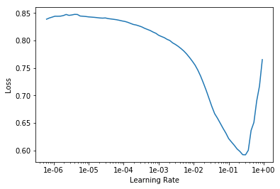
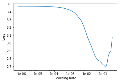
One thing to notice here is that before we unfreeze you'll tend to get this shape pretty much all the time:

If you do your learning rate finder before you unfreeze. It's pretty easy ﹣ find the steepest slope, not the bottom. Remember, we're trying to find the bit where we can like slide down it quickly. So if you start at the bottom it's just gonna send you straight off to the end here.

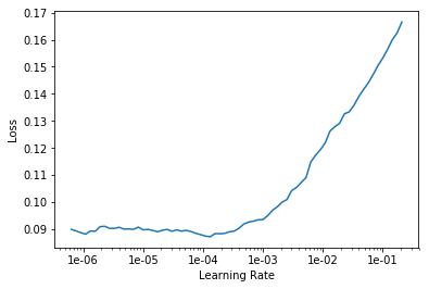
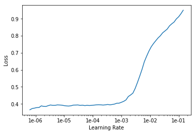
Then we can call it again after you unfreeze, and you generally get a very different shape.

49:24

This is a little bit harder to say what to look for because it tends to be this kind of shape where you get a little bit of upward and then it kind of very gradual downward and then up here. So I tend to kind of look for just before it shoots up and go back about 10x as a kind of a rule of thumb. So one 1e-5. That is what I do for the first half of my slice. And then for the second half of my slice, I normally do whatever learning rate are used for the the frozen part. So lr which was 0.01 kind of divided by five or ten. Somewhere around that. That's my rule of thumb:

look for the bit kind of at the bottom find about 10x smaller that's the number that I put as the first half of my slice
lr/5 or lr/10 is kind of what I put as the second half of my slice

This is called discriminative learning rates as the course continues.

Making the model better [50:30]

How am I going to get this better? We want to get into the top 10% which is going to be about 0.929 ish so we're not quite there (0.9288).

So here's the trick [51:01]. When I created my dataset, I put size=128 and actually the images that Kaggle gave us are 256. I used the size of 128 partially because I wanted to experiment quickly. It's much quicker and easier to use small images to experiment. But there's a second reason. I now have a model that's pretty good at recognizing the contents of 128 by 128 satellite images. So what am I going to do if I now want to create a model that's pretty good at 256 by 256 satellite images? Why don't I use transfer learning? Why don't I start with the model that's good at 128 by 128 images and fine-tune that? So don't start again. That's actually going to be really interesting because if I trained quite a lot and I'm on the verge of overfitting then I'm basically creating a whole new dataset effectively﹣one where my images are twice the size on each axis right so four times bigger. So it's really a totally different data set as far as my convolutional neural networks concerned. So I got to lose all that overfitting. I get to start again. Let's keep our same learner but use a new data bunch where the data bunch is 256 by 256. That's why I actually stopped here before I created my data sets:

Because I'm going to now take this this data source (src) and I'm going to create a new data bunch with 256 instead so let's have a look at how we do that.

data = (src.transform(tfms, size=256)
        .databunch().normalize(imagenet_stats))

So here it is. Take that source, transform it with the same transforms as before but this time use size 256. That should be better anyway because this is going to be higher resolution images. But also I'm going to start with this kind of pre-trained model (I haven't got rid of my learner it's the same learner I had before).

I'm going to replace the data inside my learner with this new data bunch.

learn.data = data
data.train_ds[0][0].shape

torch.Size([3, 256, 256])

learn.freeze()

Then I will freeze again (i.e. I'm going back to just training the last few layers) and I will do a new lr_find().

learn.lr_find()
learn.recorder.plot()

Because I actually now have a pretty good model (it's pretty good for 128 by 128 so it's probably gonna be like at least okay for 256 by 256), I don't get that same sharp shape that I did before. But I can certainly see where it's way too high. So I'm gonna pick something well before where it's way too high. Again maybe 10x smaller. So here I'm gonna go 1e-2/2 ﹣ that seems well before it shoots up.

lr=1e-2/2

So let's fit a little bit more.

learn.fit_one_cycle(5, slice(lr))

Total time: 14:21
epoch  train_loss  valid_loss  accuracy_thresh  fbeta
    0.088628    0.085883    0.966523         0.924035  (02:53)
    0.089855    0.085019    0.967126         0.926822  (02:51)
    0.083646    0.083374    0.967583         0.927510  (02:51)
    0.084014    0.081384    0.968405         0.931110  (02:51)
    0.083445    0.081085    0.968659         0.930647  (02:52)

We frozen again so we're just trading the last few layers and fit a little bit more. As you can see, I very quickly remember 0.928 was where we got to before after quite a few epochs. we're straight up there and suddenly we've passed 0.93. So we're now already into the top 10%. So we've hit our first goal. We're, at the very least, pretty confident at the problem of recognizing satellite imagery.

learn.save('stage-1-256-rn50')

But of course now, we can do the same thing as before. We can unfreeze and train a little more.

learn.unfreeze()

Again using the same kind of approach I described before lr/5 on the right and even smaller one on the left.

learn.fit_one_cycle(5, slice(1e-5, lr/5))

Total time: 18:23
epoch  train_loss  valid_loss  accuracy_thresh  fbeta
    0.083591    0.082895    0.968310         0.928210  (03:41)
    0.088286    0.083184    0.967424         0.928812  (03:40)
    0.083495    0.083084    0.967998         0.929224  (03:40)
    0.080143    0.081338    0.968564         0.931363  (03:40)
    0.074927    0.080691    0.968819         0.931414  (03:41)

Train a little bit more. 0.9314 so that's actually pretty good﹣somewhere around top 25ish. Actually when my friend Brendan and I entered this competition we came 22nd with 0.9315 and we spent (this was a year or two ago) months trying to get here. So using pretty much defaults with the minor tweaks and one trick which is the resizing tweak you can get right up into the top of the leaderboard of this very challenging competition. Now I should say we don't really know where we'd be﹣we would actually have to check it on the test set that Kaggle gave us and actually submit to the competition which you can do. You can do a late submission. So later on in the course, we'll learn how to do that. But we certainly know we're doing very well so that's great news.

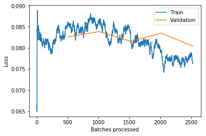
learn.recorder.plot_losses()

learn.save('stage-2-256-rn50')

You can see as I kind of go along I tend to save things. You can name your models whatever you like but I just want to basically know you know is it before or after the unfreeze (stage 1 or 2), what size was I training on, what architecture was I training on. That way I could have always go back and experiment pretty easily. So that's planet. Multi-label classification.

Segmentation example and CamVid [56:31]

lesson3-camvid.ipynb

The next example we're going to look at is this dataset called CamVid. It's going to be doing something called segmentation. We're going to start with a picture like the left:

and we're going to try and create a color-coded picture like the right where all of the bicycle pixels are the same color all of the road line pixels are the same color all of the tree pixels of the same color all of the building pixels are same color the sky the same color and so forth.

Now we're not actually going to make them colors, we're actually going to do it where each of those pixels has a unique number. In this case the top of left is building, so I guess building this number 4, the top right is tree, so tree is 26, and so forth.

In other words, this single top left pixel, we're going to do a classification problem just like the pet's classification for the very top left pixel. We're going to say "what is that top left pixel? Is it bicycle, road lines, sidewalk, building?" Then what is the next pixel along? So we're going to do a little classification problem for every single pixel in every single image. That's called segmentation.

In order to build a segmentation model, you actually need to download or create a dataset where someone has actually labeled every pixel. As you can imagine, that's a lot of work, so you're probably not going to create your own segmentation datasets but you're probably going to download or find them from somewhere else.

This is very common in medicine and life sciences. If you're looking through slides at nuclei, it's very likely you already have a whole bunch of segmented cells and segmented nuclei. If you're in radiology, you probably already have lots of examples of segmented lesions and so forth. So there's a lot of different domain areas where there are domain-specific tools for creating these segmented images. As you could guess from this example, it's also very common in self-driving cars and stuff like that where you need to see what objects are around and where are they.

In this case, there's a nice dataset called CamVid which we can download and they have already got a whole bunch of images and segment masks prepared for us. Remember, pretty much all of the datasets that we have provided inbuilt URLs for, you can see their details at https://course.fast.ai/datasets and nearly all of them are academic datasets where some very kind people have gone to all of this trouble for us so that we can use this dataset and made it available for us to use. So if you do use one of these datasets for any kind of project, it would be very very nice if you were to go and find the citation and say "thanks to these people for this dataset." Because they've provided it and all they're asking in return is for us to give them that credit. So here is the CamVid dataset and the citation (on our data sets page, that will link to the academic paper where it came from).

Question: Is there a way to use learn.lr_find() and have it return a suggested number directly rather than having to plot it as a graph and then pick a learning rate by visually inspecting that graph? (And there are a few other questions around more guidance on reading the learning rate finder graph) [1:00:26]

The short answer is no and the reason the answer is no is because this is still a bit more artisinal than I would like. As you can see, I've been saying how I read this learning rate graph depends a bit on what stage I'm at and what the shape of it is. I guess when you're just training the head (so before you unfreeze), it pretty much always looks like this:

And you could certainly create something that creates a smooth version of this, finds the sharpest negative slope and picked that you would probably be fine nearly all the time.

But then for you know these kinds of ones, it requires a certain amount of experimentation:

But the good news is you can experiment. Obviously if the lines going up, you don't want it. Almost certainly at the very bottom point, you don't want it right because you needed to be going downwards. But if you kind of start with somewhere around 10x smaller than that, and then also you could try another 10x smaller than that, try a few numbers and find out which ones work best.

And within a small number of weeks, you will find that you're picking the best learning rate most of the time. So at this stage, it still requires a bit of playing around to get a sense of the different kinds of shapes that you see and how to respond to them. Maybe by the time this video comes out, someone will have a pretty reliable auto learning rate finder. We're not there yet. It's probably not a massively difficult job to do. It would be an interesting project﹣collect a whole bunch of different datasets, maybe grab all the datasets from our datasets page, try and come up with some simple heuristic, compare it to all the different lessons I've shown. It would be a really fun project to do. But at the moment, we don't have that. I'm sure it's possible but we haven't got them.

📝 a fun project to do is create a reliable auto learning rate finder.

Image Segmentation with CamVid [1:03:05]

So how do we do image segmentation? The same way we do everything else. Basically we're going to start with some path which has got some information in it of some sort.

%reload_ext autoreload
%autoreload 2
%matplotlib inline

from fastai import *
from fastai.vision import *

So I always start by un-taring my data, do an ls, see what I was given. In this case there's a label a folder called labels and a folder called images, so I'll create paths for each of those.

path = untar_data(URLs.CAMVID)
path.ls()

[PosixPath('/home/ubuntu/course-v3/nbs/dl1/data/camvid/images'),
 PosixPath('/home/ubuntu/course-v3/nbs/dl1/data/camvid/codes.txt'),
 PosixPath('/home/ubuntu/course-v3/nbs/dl1/data/camvid/valid.txt'),
 PosixPath('/home/ubuntu/course-v3/nbs/dl1/data/camvid/labels')]

path_lbl = path/'labels'
path_img = path/'images'

We'll take a look inside each of those.

fnames = get_image_files(path_img)
fnames[:3]

[PosixPath('/home/ubuntu/course-v3/nbs/dl1/data/camvid/images/0016E5_08370.png'),
 PosixPath('/home/ubuntu/course-v3/nbs/dl1/data/camvid/images/Seq05VD_f04110.png'),
 PosixPath('/home/ubuntu/course-v3/nbs/dl1/data/camvid/images/0001TP_010170.png')]

lbl_names = get_image_files(path_lbl)
lbl_names[:3]

[PosixPath('/home/ubuntu/course-v3/nbs/dl1/data/camvid/labels/0016E5_01890_P.png'),
 PosixPath('/home/ubuntu/course-v3/nbs/dl1/data/camvid/labels/Seq05VD_f00330_P.png'),
 PosixPath('/home/ubuntu/course-v3/nbs/dl1/data/camvid/labels/Seq05VD_f01140_P.png')]

You can see there's some kind of coded file names for the images and some kind of coded file names for the segment masks. Then you kind of have to figure out how to map from one to the other. Normally, these kind of datasets will come with a README you can look at or you can look at their website.

img_f = fnames[0]
img = open_image(img_f)
img.show(figsize=(5,5))

get_y_fn = lambda x: path_lbl/f'{x.stem}_P{x.suffix}'

Often it's obvious﹣in this case I just guessed. I thought it's probably the same thing _P, so I created a little function that basically took the filename and added the _P and put it in the different place (path_lbl) and I tried opening it and I noticed it worked.

mask = open_mask(get_y_fn(img_f))
mask.show(figsize=(5,5), alpha=1)

So I've created this little function that converts from the image file names to the equivalent label file names. I opened up that to make sure it works. Normally, we use open_image to open a file and then you can go .show to take a look at it, but as we described, this is not a usual image file that contains integers. So you have to use open_masks rather than open_image because we want to return integers not floats. Fastai knows how to deal with masks, so if you go mask.show, it will automatically color code it for you in some appropriate way. That's why we said open_masks.

src_size = np.array(mask.shape[1:])
src_size,mask.data

(array([720, 960]), tensor([[[30, 30, 30,  ...,  4,  4,  4],
          [30, 30, 30,  ...,  4,  4,  4],
          [30, 30, 30,  ...,  4,  4,  4],
          ...,
          [17, 17, 17,  ..., 17, 17, 17],
          [17, 17, 17,  ..., 17, 17, 17],
          [17, 17, 17,  ..., 17, 17, 17]]]))

We can kind of have a look inside look at the data see what the size is so there's 720 by 960. We can take a look at the data inside, and so forth. The other thing you might have noticed is that they gave us a file called codes.txt and a file called valid.txt.

codes = np.loadtxt(path/'codes.txt', dtype=str); codes

array(['Animal', 'Archway', 'Bicyclist', 'Bridge', 'Building', 'Car', 'CartLuggagePram', 'Child', 'Column_Pole',
       'Fence', 'LaneMkgsDriv', 'LaneMkgsNonDriv', 'Misc_Text', 'MotorcycleScooter', 'OtherMoving', 'ParkingBlock',
       'Pedestrian', 'Road', 'RoadShoulder', 'Sidewalk', 'SignSymbol', 'Sky', 'SUVPickupTruck', 'TrafficCone',
       'TrafficLight', 'Train', 'Tree', 'Truck_Bus', 'Tunnel', 'VegetationMisc', 'Void', 'Wall'], dtype='<U17')

code.txt contains a list telling us that, for example, number 4 isbuilding. Just like we had grizzlies, black bears, and teddies, here we've got the coding for what each one of these pixels means.

Creating a data bunch [1:05:53]

To create a data bunch, we can go through the Data Block API and say:

We've got a list of image files that are in a folder
We then need to split into training and validation. In this case I don't do it randomly because the pictures they've given us are frames from videos. If I did them randomly I would be having two frames next to each other: one in the validation set, one in the training set. That would be far too easy and treating. So the people that created this dataset actually gave us a list of file names (valid.txt) that are meant to be in your validation set and they are non-contiguous parts of the video. So here's how you can split your validation and training using a file name file.
We need to create labels which we can use that get_y_fn (get Y file name function) we just created .

size = src_size//2
bs=8

src = (SegmentationItemList.from_folder(path_img)
       .split_by_fname_file('../valid.txt')
       .label_from_func(get_y_fn, classes=codes))

From that, I can create my datasets.

So I actually have a list of class names. Often with stuff like the Planet dataset or the pets dataset, we actually have a string saying this is a pug, this is a ragdoll, or this is a birman, or this is cloudy or whatever. In this case, you don't have every single pixel labeled with an entire string (that would be incredibly inefficient). They're each labeled with just a number and then there's a separate file telling you what those numbers mean. So here's where we get to tell the Data Block API this is the list of what the numbers mean. So these are the kind of parameters that the Data Block API gives you.

data = (src.transform(get_transforms(), size=size, tfm_y=True)
        .databunch(bs=bs)
        .normalize(imagenet_stats))

Here's our transformations. Here's an interesting point. Remember I told you that, for example, sometimes we randomly flip an image? What if we randomly flip the independent variable image but we don't also randomly flip the target mask? Now I'm not matching anymore. So we need to tell fastai that I want to transform the Y (X is our independent variable, Y is our dependent)﹣I want to transform the Y as well. So whatever you do to the X, I also want you to do to the Y (tfm_y=True). There's all these little parameters that we can play with.

I can create our data bunch. I'm using a smaller batch size (bs=8) because, as you can imagine, I'm creating a classifier for every pixel, that's going to take a lot more GPU right. I found a batch size of 8 is all I could handle. Then normalize in the usual way.

data.show_batch(2, figsize=(10,7))

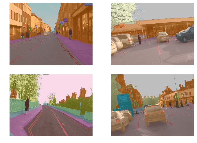
This is quite nice. Because fastai knows that you've given it a segmentation problem, when you call show batch, it actually combines the two pieces for you and it will color code the photo. Isn't that nice? So this is what the ground truth data looks.

Training [1:09:00]

Once we've got that, we can go ahead and

Create a learner. I'll show you some more details in a moment.
Call lr_find, find the sharpest bit which looks about 1e-2.
Call fit passing in slice(lr) and see the accuracy.
Save the model.
Unfreeze and train a little bit more.

That's the basic idea.

name2id = {v:k for k,v in enumerate(codes)}
void_code = name2id['Void']

def acc_camvid(input, target):
    target = target.squeeze(1)
    mask = target != void_code
    return (input.argmax(dim=1)[mask]==target[mask]).float().mean()

metrics=acc_camvid
# metrics=accuracy

learn = Learner.create_unet(data, models.resnet34, metrics=metrics)

lr_find(learn)
learn.recorder.plot()

lr=1e-2

learn.fit_one_cycle(10, slice(lr))

Total time: 02:46
epoch  train_loss  valid_loss  acc_camvid
    1.537235    0.785360    0.832015    (00:20)
    0.905632    0.677888    0.842743    (00:15)
    0.755041    0.759045    0.844444    (00:16)
    0.673628    0.522713    0.854023    (00:16)
    0.603915    0.495224    0.864088    (00:16)
    0.557424    0.433317    0.879087    (00:16)
    0.504053    0.419078    0.878530    (00:16)
    0.457378    0.371296    0.889752    (00:16)
    0.428532    0.347722    0.898966    (00:16)
   0.409673    0.341935    0.901897    (00:16)

learn.save('stage-1')

learn.load('stage-1');

learn.unfreeze()

lr_find(learn)
learn.recorder.plot()

lrs = slice(1e-5,lr/5)

learn.fit_one_cycle(12, lrs)

Total time: 03:36
epoch  train_loss  valid_loss  acc_camvid
    0.399582    0.338697    0.901930    (00:18)
    0.406091    0.351272    0.897183    (00:18)
    0.415589    0.357046    0.894615    (00:17)
    0.407372    0.337691    0.904101    (00:18)
    0.402764    0.340527    0.900326    (00:17)
    0.381159    0.317680    0.910552    (00:18)
    0.368179    0.312087    0.910121    (00:18)
    0.358906    0.310293    0.911405    (00:18)
    0.343944    0.299595    0.912654    (00:18)
   0.332852    0.305770    0.911666    (00:18)
   0.325537    0.294337    0.916766    (00:18)
   0.320488    0.295004    0.916064    (00:18)

Announcement: 📢 there's been one change to fastai v1.0.29 (2018-11-27) and above—Learner.create_unet is now called unet_learner.

Question: Could you use unsupervised learning here (pixel classification with the bike example) to avoid needing a human to label a heap of images? [1:10:03]

Not exactly unsupervised learning, but you can certainly get a sense of where things are without needing these kind of labels. Time permitting, we'll try and see some examples of how to do that. You're certainly not going to get as such a quality and such a specific output as what you see here though. If you want to get this level of segmentation mask, you need a pretty good segmentation mask ground truth to work with.

Question: Is there a reason we shouldn’t deliberately make a lot of smaller datasets to step up from in tuning? let’s say 64x64, 128x128, 256x256, etc… [1:10:51]

Yes, you should totally do that. It works great. This idea, it's something that I first came up with in the course a couple of years ago and I thought it seemed obvious and just presented it as a good idea, then I later discovered that nobody had really published this before. And then we started experimenting with it. And it was basically the main tricks that we use to win the DAWNBench ImageNet training competition.

Not only was this not standard, but nobody had heard of it before. There's been now a few papers that use this trick for various specific purposes but it's still largely unknown. It means that you can train much faster, it generalizes better. There's still a lot of unknowns about exactly how small, how big, and how much at each level and so forth. We call it "progressive resizing". I found that going much under 64 by 64 tends not to help very much. But yeah, it's a great technique and I definitely try a few a few different sizes.

Question: [1:12:35] What does accuracy mean for pixel wise segmentation? Is it

#correctly classified pixels / #total number of pixels?

Yep, that's it. So if you imagined each pixel was a separate object you're classifying, it's exactly the same accuracy. So you actually can just pass in accuracy as your metric, but in this case, we actually don't. We've created a new metric called acc_camvid and the reason for that is that when they labeled the images, sometimes they labeled a pixel as Void. I'm not quite sure why but some of the pixels are Void. And in the CamVid paper, they say when you're reporting accuracy, you should remove the void pixels. So we've created a accuracy CamVid. so all metrics take the actual output of the neural net (i.e. that's the input to the metric) and the target (i.e. the labels we are trying to predict).

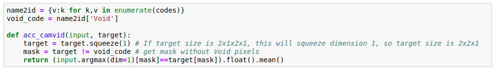
We then basically create a mask (we look for the places where the target is not equal to Void) and then we just take the input, do the argmax as per usual, but then we just grab those that are not equal to the void code. We do the same for the target and we take the mean, so it's just a standard accuracy.

It's almost exactly the same as the accuracy source code we saw before with the addition of this mask. This quite often happens. The particular Kaggle competition metric you're using or the particular way your organization scores things, there's often little tweaks you have to do. And this is how easy it is. As you'll see, to do this stuff, the main thing you need to know pretty well is how to do basic mathematical operations in PyTorch so that's just something you kind of need to practice.

Question: I've noticed that most of the examples and most of my models result in a training loss greater than the validation loss. What are the best ways to correct that? I should add that this still happens after trying many variations on number of epochs and learning rate. [1:15:03]

Good question. Remember from last week, if you're training loss is higher than your validation loss then you're underfitting. It definitely means that your underfitting. You want your training loss to be lower than your validation loss. If you're underfitting, you can:

Train for longer.
Train the last bit at a lower learning rate.

But if you're still under fitting, then you're going to have to decrease regularization. We haven't talked about that yet. In the second half of this part of the course, we're going to be talking quite a lot about regularization and specifically how to avoid overfitting or underfitting by using regularization. If you want to skip ahead, we're going to be learning about:

weight decay
dropout
data augmentation

They will be the key things that are we talking about.

U-Net [1:16:24]

For segmentation, we don't just create a convolutional neural network. We can, but actually an architecture called U-Net turns out to be better.

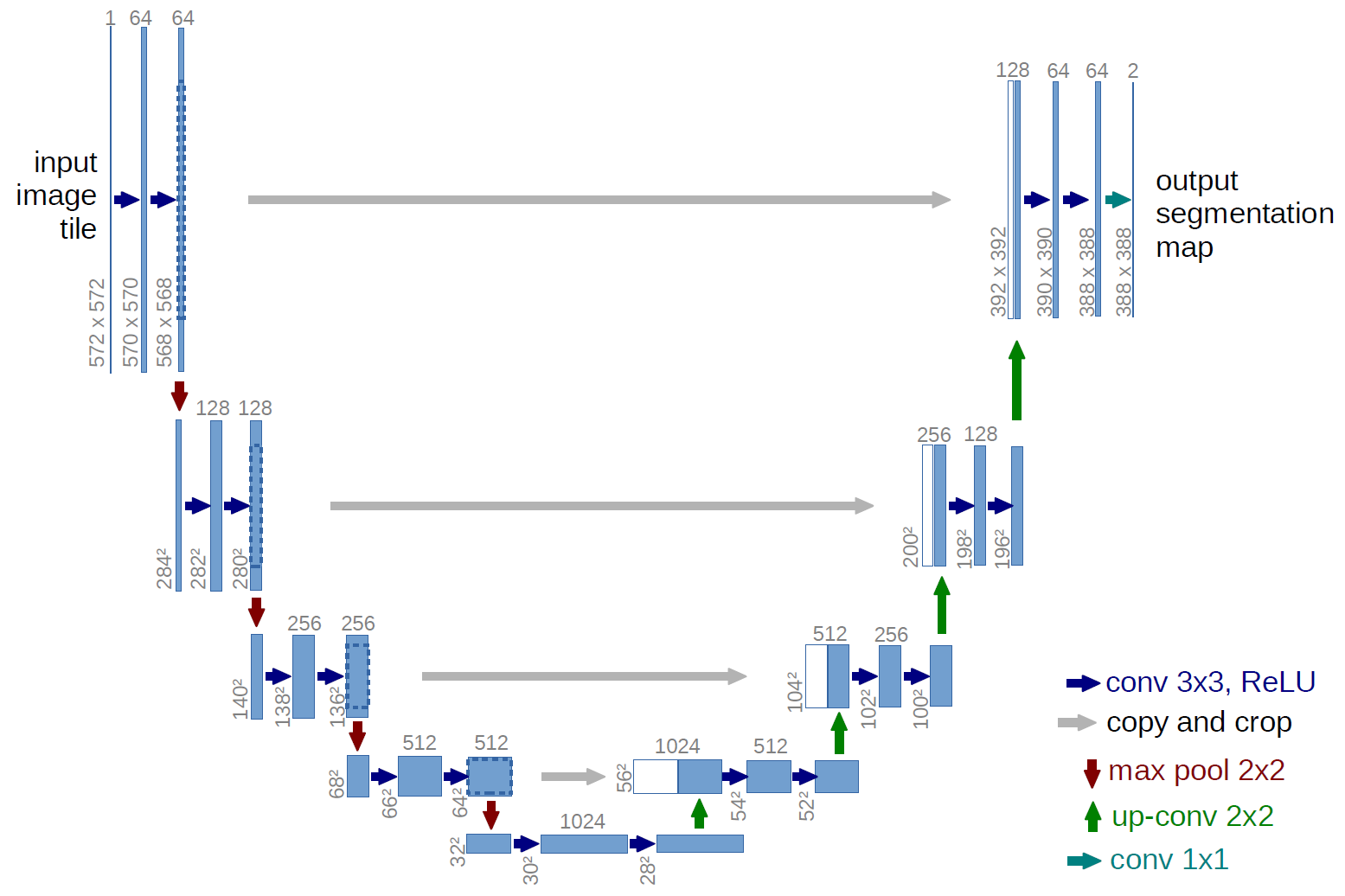
This is what a U-Net looks like. This is from the University website where they talk about the U-Net. So we'll be learning about this both in this part of the course and in part two if you do it. But basically this bit down on the left hand side is what a normal convolutional neural network looks like. It's something which starts with a big image and gradually makes it smaller and smaller until eventually you just have one prediction. What a U-Net does is it then takes that and makes it bigger and bigger and bigger again, and then it takes every stage of the downward path and copies it across, and it creates this U shape.

It's was originally actually created/published as a biomechanical image segmentation method. But it turns out to be useful for far more than just biomedical image segmentation. It was presented at MICCAI which is the main medical imaging conference, and as of just yesterday, it actually just became the most cited paper of all time from that conference. So it's been incredibly useful﹣over 3,000 citations.

You don't really need to know any details at this stage. All you need to know is if you want to create a segmentation model, you want to be saying Learner.create_unet rather than create_cnn. But you pass it the normal stuff: their data bunch, architecture, and some metrics.

Having done that, everything else works the same.

A little more about `learn.recorder` [1:18:54]

Here's something interesting. learn.recorder is where we keep track of what's going on during training. It's got a number nice methods one of which is plot losses.

learn.recorder.plot_losses()

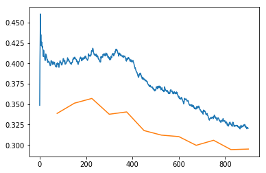
learn.recorder.plot_lr()

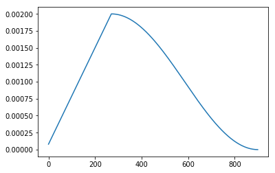
This plots your training loss and your validation loss. Quite often, they actually go up a bit before they go down. Why is that? That's because (you can also plot your learning rate over time and you'll see that) the learning rate goes up and then it goes down. Why is that? Because we said fit_one_cycle. That's what fit one cycle does. It actually makes the learning rate start low, go up, and then go down again.

Why is that a good idea? To find out why that's a good idea, let's first of all look at a really cool project done by José Fernández Portal during the week. He took our gradient descent demo notebook and actually plotted the weights over time, not just the ground truth and model over time. He did it for a few different learning rates.

Remember we had two weights we were doing basically $y=ax+b$ or in his nomenclature $y=w_{0}x+w_{1}$ .

We can actually look and see what happens to those weights over time. And we know this is the correct answer (marked with red X). A learning rate of 0.1, they're kind of like slides on in here and you can see that it takes a little bit of time to get to the right point. You can see the loss improving.

At a higher learning rate of 0.7, you can see that the model jumps to the ground truth really quickly. And you can see that the weights jump straight to the right place really quickly:

What if we have a learning rate that's really too high you can see it takes a very very long time to get to the right point:

Or if it's really too high, it diverges:

So you can see why getting the right learning rate is important. When you get the right learning rate, it zooms into the best spot very quickly.

Now as you get closer to the final spot, something interesting happens which is that you really want your learning rate to decrease because you're getting close to the right spot.

So what actually happens is (I can only draw 2d sorry), you don't generally have some kind of loss function surface that looks like that (remember there's lots of dimensions), but it actually tends to look bumpy like that. So you want a learning rate that's like high enough to jump over the bumps, but once you get close to the best answer, you don't want to be just jumping backwards and forwards between bumps. You want your learning rate to go down so that as you get closer, you take smaller and smaller steps. That's why it is that we want our learning rate to go down at the end.

This idea of decreasing the learning rate during training has been around forever. It's just called learning rate annealing. But the idea of gradually increasing it at the start is much more recent and it mainly comes from a guy called Leslie Smith (meetup with Leslie Smith).

Loss function surfaces tend have flat areas and bumpy areas. If you end up in the bottom of a bumpy area, that solution will tend not to generalize very well because you've found a solution that's good in that one place but it's not very good in other places. Where else if you found one in the flat area, it probably will generalize well because it's not only good in that one spot but it's good to kind of around it as well.

If you have a really small learning rate, it'll tend to kind of plud down and stick in these places. But if you gradually increase the learning rate, then it'll kind of like jump down and as the learning rate goes up, it's going to start going up again like this. Then the learning rate is now going to be up here, it's going to be bumping backwards and forwards. Eventually the learning rate starts to come down again, and it'll tend to find its way to these flat areas.

So it turns out that gradually increasing the learning rate is a really good way of helping the model to explore the whole function surface, and try and find areas where both the loss is low and also it's not bumpy. Because if it was bumpy, it would get kicked out again. This allows us to train at really high learning rates, so it tends to mean that we solve our problem much more quickly, and we tend to end up with much more generalizable solutions.

What you are looking for in `plot_losses` [1:25:01]

If you call plot_losses and find that it's just getting a little bit worse and then it gets a lot better you've found a really good maximum learning rate.

So when you actually call fit one cycle, you're not actually passing in a learning rate. You're actually passing in a maximum learning rate. if it's kind of always going down, particularly after you unfreeze, that suggests you could probably bump your learning rates up a little bit﹣because you really want to see this kind of shape. It's going to train faster and generalize better. You'll to tend to particularly see it in the validation set (the orange is the validation set). Again, the difference between kind of knowing this theory and being able to do it, is looking at lots of these pictures. So after you train stuff, type learn.recorder. and hit tab, and see what's in there﹣particularly the things that start with "plot" and start getting a sense of what are these pictures looking like when you're getting good results. Then try making the learning rate much higher, try making it much lower, more epochs, less epochs, and get a sense for what these look like.

Go big [1:26:16]

In this case, we used the size (in our transforms) of the original image size/2. These two slashes in Python means integer divide because obviously we can't have half pixel amounts in our sizes. We use the batch size of 8. Now I found that fits on my GPU, it might not fit on yours. If it doesn't, you can just decrease the batch size down to 4.

This isn't really solving the problem because the problem is to segment all of the pixels﹣not half of the pixels. So I'm going to use the same trick that I did last time which is I'm now going to put the size up to the full size of the source images which means I now have to halve my batch size otherwise I'll run out of GPU memory.

size = src_size
bs=4

data = (src.transform(get_transforms(), size=size, tfm_y=True)
        .databunch(bs=bs)
        .normalize(imagenet_stats))

learn = Learner.create_unet(data, models.resnet34, metrics=metrics)

learn.load('stage-2');

I can either say learn.data = data but I actually found it had a lot of trouble with GPU memory, so I generally restarted my kernel, came back here, created a new learner, and loaded up the weights that I saved last time.

The key thing is that this learner now has the same weights that I had before, but the data is now the full image size.

lr_find(learn)
learn.recorder.plot()

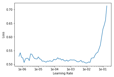
lr=1e-3

learn.fit_one_cycle(10, slice(lr))

Total time: 08:44
epoch  train_loss  valid_loss  acc_camvid
    0.454597    0.349557    0.900428    (01:02)
    0.418897    0.351502    0.897495    (00:51)
    0.402104    0.330255    0.906775    (00:50)
    0.385497    0.313330    0.911832    (00:51)
    0.359252    0.297264    0.916108    (00:52)
    0.335910    0.297875    0.917553    (00:50)
    0.336133    0.305602    0.913439    (00:51)
    0.321016    0.305374    0.914063    (00:51)
    0.311554    0.299226    0.915997    (00:51)
   0.308389    0.301060    0.915253    (00:51)

learn.save('stage-1-big')

learn.load('stage-1-big');

learn.unfreeze()

lrs = slice(1e-6,lr)

learn.fit_one_cycle(10, lrs, wd=1e-3)

Total time: 09:30
epoch  train_loss  valid_loss  acc_camvid
    0.323283    0.300749    0.915948    (00:56)
    0.329482    0.290447    0.918337    (00:56)
    0.324378    0.298494    0.920271    (00:57)
    0.316414    0.296469    0.918053    (00:56)
    0.305226    0.284694    0.920893    (00:57)
    0.301774    0.306676    0.914202    (00:57)
    0.279722    0.285487    0.919991    (00:57)
    0.269306    0.285219    0.920963    (00:57)
    0.260325    0.284758    0.922026    (00:57)
   0.251017    0.285375    0.921562    (00:57)

learn.save('stage-2-big')

learn.load('stage-2-big')

learn.show_results()

You can go learn.show_results() to see how your predictions compare to the ground truth, and they really look pretty good.

How good is pretty good? An accuracy of 92.15%, the best paper I know of for segmentation was a paper called The One Hundred Layers Tiramisu which developed a convolutional dense net came out about two years ago. After I trained this today, I went back and looked at the paper to find their state-of-the-art accuracy and their best was 91.5% and we got 92.1%. I don't know if better results have come out since this paper, but I remember when this paper came out and it was a really big deal. I said "wow, this this is an exceptionally good segmentation result." When you compare it to the previous bests that they compared it to it was a big step up.

In last year's course, we spent a lot of time re-implementing the hundred layers tiramisu. Now with our totally default fastai class, and it's easily beating 91.5%. I also remember I had to train for hours and hours. Where else, today's version, I trained in minutes. So this is a super strong architecture for segmentation.

I'm not going to promise that this is the definite state-of-the-art today, because I haven't done a complete literature search to see what's happened in the last two years. But it's certainly beating the world's best approach the last time I looked into this which was in last year's course basically. So these are all the little tricks we've picked up along the way in terms of how to train things well: things like using the pre-trained model and the one cycle convergence. All these little tricks they work extraordinarily well.

We actually haven't published the paper on the exact details of how this variation of the U-Net works﹣there's a few little tweaks we do, but if you come back for part 2, we'll be going into all of the details about how we make this work so well. But for you, all you have to know at this stage is that you can say learner.create_unet and you should get great results also.

Another trick: Mixed precision training [1:30:59]

There's another trick you can use if you're running out of memory a lot which is you can actually do something called mixed precision training. Mixed precision training means that (for those of you that have done a little bit of computer science) instead of using single precision floating point numbers, you can do most of the calculations in your model with half precision floating point numbers﹣so 16 bits instead of 32 bits. The very idea of this has only been around for the last couple of years﹣in terms of like hardware that actually does this reasonably quickly. Then fastai library, I think, is the first and probably still the only that makes it actually easy to use this.

If you add to_fp16() on the end of any learner call, you're actually going to get a model that trains in 16-bit precision. Because it's so new, you'll need to have the most recent CUDA drivers and all that stuff for this even to work. When I tried it this morning on some of the platforms, it just killed the kernel, so you need to make sure you've got the most recent drivers. If you've got a really recent GPU like 2080Ti, not only will it work, but it'll work about twice as fast as otherwise. The reason I'm mentioning it is that it's going to use less GPU RAM, so even if you don't have a 2080Ti, you'll probably find that things that didn't fit into your GPU without this do fit in.

I actually have never seen people use mixed precision floating point for segmentation before, just for a bit of a laugh I tried it and actually discovered that I got even better result. I only found this this morning so I don't have anything more to add here rather than quite often when you make things a little bit less precise in deep learning, it generalizes a little bit better. I've never seen a 92.5% accuracy on CamVid before, so not only will this be faster, you'll be able to use bigger batch sizes, but you might even find like I did that you get an even better result. So that's a cool little trick.

You just need to make sure that every time you create a learner you add at this to_fp16(). If your kernel dies, it probably means you have slightly out of date CUDA drivers or maybe even a too old graphics card I'm not sure exactly which cards support FP16.

Regression with BIWI head pose dataset [1:34:03]

lesson3-head-pose.ipynb

Two more before we kind of rewind. The first one I'm going to show you is an interesting data set called the BIWI head pose dataset. Gabriele Fanelli was kind enough to give us permission to use this in the class. His team created this cool dataset.

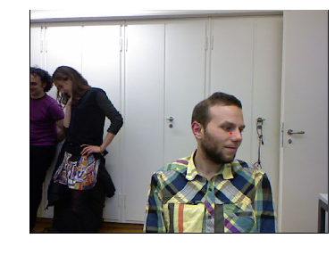
Here's what the data set looks like. It's actually got a few things in it. We're just going to do a simplified version, and one of the things they do is they have a dot saying this is the center of the face. So we're going to try and create a model that can find this ever face.

%reload_ext autoreload
%autoreload 2
%matplotlib inline

from fastai import *
from fastai.vision import *

For this dataset, there's a few dataset specific things we have to do which I don't really even understand but I just know from the readme that you have to. They use some kind of depth sensing camera, I think they actually use Xbox Kinect.

path = untar_data(URLs.BIWI_HEAD_POSE)

There's some kind of calibration numbers that they provide in a little file which I had to read in:

cal = np.genfromtxt(path/'01'/'rgb.cal', skip_footer=6); cal

array([[517.679,   0.   , 320.   ],
       [  0.   , 517.679, 240.5  ],
       [  0.   ,   0.   ,   1.   ]])

fname = '09/frame_00667_rgb.jpg'

def img2txt_name(f): return path/f'{str(f)[:-7]}pose.txt'

img = open_image(path/fname)
img.show()

ctr = np.genfromtxt(img2txt_name(fname), skip_header=3); ctr

array([187.332 ,  40.3892, 893.135 ])

Then they provided a little function that you have to use to take their coordinates to change it from this depth sensor calibration thing to end up with actual coordinates.

def convert_biwi(coords):
    c1 = coords[0] * cal[0][0]/coords[2] + cal[0][2]
    c2 = coords[1] * cal[1][1]/coords[2] + cal[1][2]
    return tensor([c2,c1])

def get_ctr(f):
    ctr = np.genfromtxt(img2txt_name(f), skip_header=3)
    return convert_biwi(ctr)

def get_ip(img,pts): return ImagePoints(FlowField(img.size, pts), scale=True)

So when you open this and you see these conversion routines, I'm just doing what they told us to do basically. It's got nothing particularly to do with deep learning to end up with this red dot.

get_ctr(fname)

tensor([263.9104, 428.5814])

ctr = get_ctr(fname)
img.show(y=get_ip(img, ctr), figsize=(6, 6))

The interesting bit really is where we create something which is not an image or an image segment but an image points. We'll mainly learn about this later in the course, but basically image points use this idea of coordinates. They're not pixel values, they're XY coordinates (just two numbers).

Here's an example for a particular image file name (09/frame_00667_rgb.jpg). The coordinates of the centre of the face are [263.9104, 428.5814]. So there's just two numbers which represent whereabouts on this picture is the center of the face. So if we're going to create a model that can find the center of a face, we need a neural network that spits out two numbers. But note, this is not a classification model. These are not two numbers that you look up in a list to find out that they're road or building or ragdoll cat or whatever. They're actual locations.

So far, everything we've done has been a classification model﹣something that created labels or classes. This, for the first time, is what we call a regression model. A lot of people think regression means linear regression, it doesn't. Regression just means any kind of model where your output is some continuous number or set of numbers. So we need to create an image regression model (i.e. something that can predict these two numbers). How do you do that? Same way as always.

data = (ImageItemList.from_folder(path)
        .split_by_valid_func(lambda o: o.parent.name=='13')
        .label_from_func(get_ctr, label_cls=PointsItemList)
        .transform(get_transforms(), tfm_y=True, size=(120,160))
        .databunch().normalize(imagenet_stats)
       )

We can actually just say:

I've got a list of image files.
It's in a folder.
I'm going to split it according to some function. So in this case, the files they gave us are from videos. So I picked just one folder (13) to be my validation set (i.e. a different person). So again, I was trying to think about how do I validate this fairly, so I said the fair validation would be to make sure that it works well on a person that it's never seen before. So my validation set is all going to be a particular person.
I want to label them using this function that we wrote that basically does the stuff that the readme says to grab the coordinates out of their text files. So that's going to give me the two numbers for every one.
Create a dataset. This data set, I just tell it what kind of data set it is ﹣ they're going to be a set of points of specific coordinates.
Do some transforms. Again, I have to say tfm_y=True because that red dot needs to move if I flip or rotate or warp.
Pick some size. I just picked a size that's going to work pretty quickly.
Create a data bunch.
Normalize it.

data.show_batch(3, figsize=(9,6)

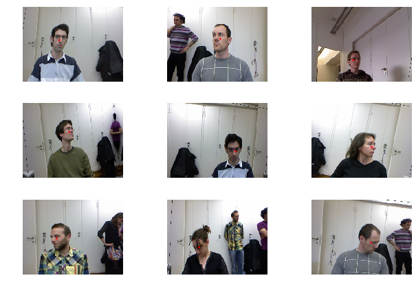
I noticed that their red dots don't always seem to be quite in the middle of the face. I don't know exactly what their internal algorithm for putting dots on. It sometimes looks like it's meant to be the nose, but sometimes it's not quite the nose. Anyway it's somewhere around the center of the face or the nose.

Create a regression model [1:38:59]

So how do we create a model? We create a CNN. We're going to be learning a lot about loss functions in the next few lessons, but basically the loss function is that number that says how good is the model. For classification, we use this loss function called cross-entropy loss which says basically "did you predict the correct class and were you confident of that prediction?" We can't use that for regression, so instead we use something called mean squared error. If you remember from last lesson, we actually implemented mean squared error from scratch. It's just the difference between the two, squared, and added up together.

learn = create_cnn(data, models.resnet34)
learn.loss_func = MSELossFlat()

So we need to tell it this is not classification so we have to use mean squared error.

learn.lr_find()
learn.recorder.plot()

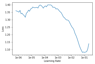
lr = 2e-2

learn.fit_one_cycle(5, slice(lr))

Total time: 07:28
epoch  train_loss  valid_loss
    0.043327    0.010848    (01:34)
    0.015479    0.001792    (01:27)
    0.006021    0.001171    (01:28)
    0.003105    0.000521    (01:27)
    0.002425    0.000381    (01:29)

Once we've created the learner, we've told it what loss function to use, we can go ahead and do lr_find, then fit and you can see here within a minute and a half our mean squared error is 0.0004.

The nice thing is about mean squared error, that's very easy to interpret. We're trying to predict something which is somewhere around a few hundred, and we're getting a squared error on average of 0.0004. So we can feel pretty confident that this is a really good model. Then we can look at the results:

learn.show_results()

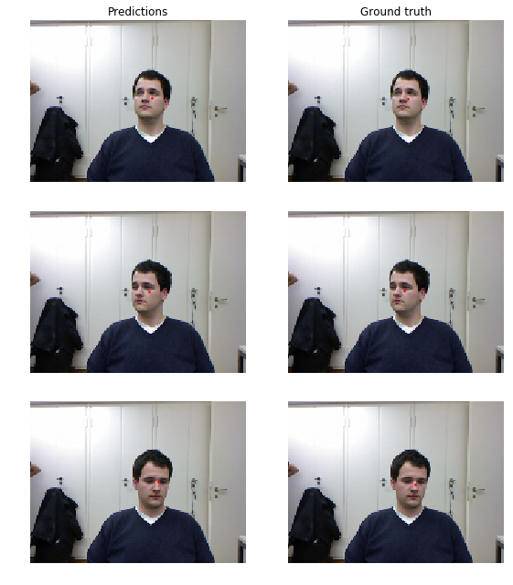
It's doing nearly perfect job. That's how you can do image regression models. Anytime you've got something you're trying to predict which is some continuous value, you use an approach that's something like this.

IMDB [1:41:07]

lesson3-imdb.ipynb

Last example before we look at more foundational theory stuff, NLP. Next week, we're going to be looking at a lot more NLP, but let's now do the same thing but rather than creating a classification of pictures, let's try and classify documents. We're going to go through this in a lot more detail next week, but let's do the quick version.

%reload_ext autoreload
%autoreload 2
%matplotlib inline

from fastai import *
from fastai.text import *

Rather than importing from fastai.vision, I now import, for the first time, from fastai.text. That's where you'll find all the application specific stuff for analyzing text documents.

In this case, we're going to use a dataset called IMDB. IMDB has lots of movie reviews. They're generally about a couple of thousand words, and each movie review has been classified as either negative or positive.

path = untar_data(URLs.IMDB_SAMPLE)
path.ls()

[PosixPath('/home/jhoward/.fastai/data/imdb_sample/texts.csv'),
 PosixPath('/home/jhoward/.fastai/data/imdb_sample/models')]

It's just in a CSV file, so we can use pandas to read it and we can take a little look.

df = pd.read_csv(path/'texts.csv')
df.head()

	label	text	is_valid
0	negative	Un-bleeping-believable! Meg Ryan doesn't even ...	False
1	positive	This is a extremely well-made film. The acting...	False
2	negative	Every once in a long while a movie will come a...	False
3	positive	Name just says it all. I watched this movie wi...	False
4	negative	This movie succeeds at being one of the most u...	False

df['text'][1]

'This is a extremely well-made film. The acting, script and camera-work are all first-rate. The music is good, too, though it is mostly early in the film, when things are still relatively cheery. There are no really superstars in the cast, though several faces will be familiar. The entire cast does an excellent job with the script.<br /><br />But it is hard to watch, because there is no good end to a situation like the one presented. It is now fashionable to blame the British for setting Hindus and Muslims against each other, and then cruelly separating them into two countries. There is some merit in this view, but it\'s also true that no one forced Hindus and Muslims in the region to mistreat each other as they did around the time of partition. It seems more likely that the British simply saw the tensions between the religions and were clever enough to exploit them to their own ends.<br /><br />The result is that there is much cruelty and inhumanity in the situation and this is very unpleasant to remember and to see on the screen. But it is never painted as a black-and-white case. There is baseness and nobility on both sides, and also the hope for change in the younger generation.<br /><br />There is redemption of a sort, in the end, when Puro has to make a hard choice between a man who has ruined her life, but also truly loved her, and her family which has disowned her, then later come looking for her. But by that point, she has no option that is without great pain for her.<br /><br />This film carries the message that both Muslims and Hindus have their grave faults, and also that both can be dignified and caring people. The reality of partition makes that realisation all the more wrenching, since there can never be real reconciliation across the India/Pakistan border. In that sense, it is similar to "Mr & Mrs Iyer".<br /><br />In the end, we were glad to have seen the film, even though the resolution was heartbreaking. If the UK and US could deal with their own histories of racism with this kind of frankness, they would certainly be better off.'

Basically as per usual, we can either use factory methods or the Data Block API to create a data bunch. So here's the quick way to create a data bunch from a CSV of texts:

data_lm = TextDataBunch.from_csv(path, 'texts.csv')

At this point I could create a learner and start training it, but we're going to show you a little bit more detail which we mainly going to look at next week. The steps that actually happen when you create these data bunches, there's a few steps:

Tokenization: it takes those words and converts them into a standard form of tokens. Basically each token represents a word.
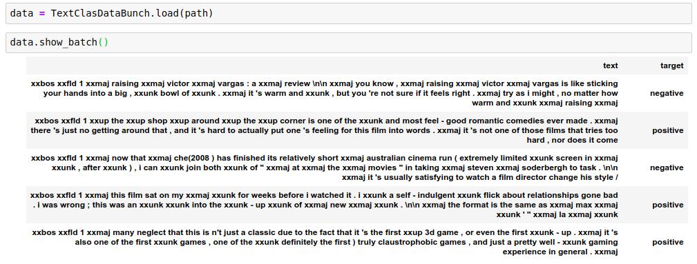
But it does things like, see how "didn't" has been turned here into two separate words (did and n't)? And everything has been lowercased. See how "you're" has been turned into two separate words (you and 're)? So tokenization is trying to make sure that each "token" (i.e. each thing that we've got with spaces around it) represents a single linguistic concept. Also it finds words that are really rare (e.g. really rare names) and replaces them with a special token called unknown (xxunk). Anything's starting with xx in fastai is some special token. This is tokenization, so we end up with something where we've got a list of tokenized words. You'll also see that things like punctuation end up with spaces around them to make sure that they're separate tokens.
Numericalization: The next thing we do is we take a complete unique list of all of the possible tokens﹣ that's called the vocab which gets created for us.
```
data.vocab.itos[:10]
```
```
['xxunk', 'xxpad', 'the', ',', '.', 'and', 'a', 'of', 'to', 'is']
```
So here is every possible token (the first ten of them) that appear in our all of the movie reviews. We then replace every movie review with a list of numbers.
```
data.train_ds[0][0].data[:10]
```
```
array([ 43,  44,  40,  34, 171,  62,   6, 352,   3,  47])
```
The list of numbers simply says what numbered thing in the vocab is in this place.

So through tokenization and numericalization, this is the standard way in NLP of turning a document into a list of numbers.

We can do that with the Data Block API:

data = (TextList.from_csv(path, 'texts.csv', cols='text')
                .split_from_df(col=2)
                .label_from_df(cols=0)
                .databunch())

This time, it's not ImageFilesList, it's TextList from a CSV and create a data bunch. At that point, we can start to create a model.

As we learn about next week, when we do NLP classification, we actually create two models:

The first model is something called a language model which we train in a kind of a usual way.
```
learn = language_model_learner(data_lm, pretrained_model=URLs.WT103, drop_mult=0.3)
```
We say we want to create a language model learner, train it, save it, and we unfreeze, train some more.
After we've created a language model, we fine-tune it to create the classifier. We create the data bunch of the classifier, create a learner, train it and we end up with some accuracy.

That's the really quick version. We're going to go through it in more detail next week, but you can see the basic idea of training and NLP classifier is very similar to creating every other model we've seen so far. The current state of the art for IMDB classification is actually the algorithm that we built and published with colleague named Sebastian Ruder and what I just showed you is pretty much the state of the art algorithm with some minor tweaks. You can get this up to about 95% if you try really hard. So this is very close to the state of the art accuracy that we developed.

Question: For a dataset very different than ImageNet like the satellite images or genomic images shown in lesson 2, we should use our own stats.

Jeremy once said:

If you’re using a pretrained model you need to use the same stats it was trained with.

Why it is that? Isn’t it that, normalized dataset with its own stats will have roughly the same distribution like ImageNet? The only thing I can think of, which may differ is skewness. Is it the possibility of skewness or something else the reason of your statement? And does that mean you don’t recommend using pre-trained model with very different dataset like the one-point mutation that you showed us in lesson 2? [1:46:53]

Nope. As you can see, I've used pre-trained models for all of those things. Every time I've used an ImageNet pre-trained model, I've used ImageNet stats. Why is that? Because that model was trained with those stats. For example, imagine you're trying to classify different types of green frogs. If you were to use your own per-channel means from your dataset, you would end up converting them to a mean of zero, a standard deviation of one for each of your red, green, and blue channels. Which means they don't look like green frogs anymore. They now look like grey frogs. But ImageNet expects frogs to be green. So you need to normalize with the same stats that the ImageNet training people normalized with. Otherwise the unique characteristics of your dataset won't appear anymore﹣you've actually normalized them out in terms of the per-channel statistics. So you should always use the same stats that the model was trained with.

In every case, what we're doing here is we're using gradient descent with mini batches (i.e. stochastic gradient descent) to fit some parameters of a model. And those parameters are parameters to matrix multiplications. The second half of this part, we're actually going to learn about a little tweak called convolutions, but it's basically a type of matrix multiplication.

The thing is though, no amount of matrix multiplications is possibly going to create something that can read IMDB movie reviews and decide if it's positive or negative or look at satellite imagery and decide whether it's got a road in it﹣that's far more than a linear classifier can do. Now we know these are deep neural networks. Deep neural networks contain lots of these matrix multiplications, but every matrix multiplication is just a linear model. A linear function on top of a linear function is just another linear function. If you remember back to your high school math, you might remember that if you have a $y = ax + b$ and then you stick another $cy + d$ on top of that, it's still just another slope and another intercept. So no amount of stacking matrix multiplications is going to help in the slightest.

So what are these models actually? What are we actually doing? And here's the interesting thing﹣all we're actually doing is we literally do have a matrix multiplication (or a slight variation like a convolution that we'll learn about) but after each one, we do something called a non-linearity or an activation function. An activation function is something that takes the result of that matrix multiplication and sticks it through some function. These are some of the functions that we use (by Sagar Sharma):

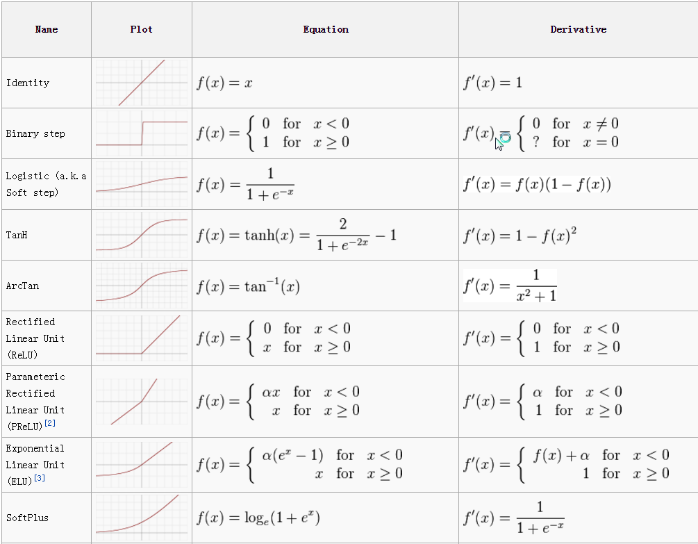
In the old days, the most common function that we used to use was sigmoid. And they have particular mathematical definitions. Nowadays, we almost never use those for these between each matrix multiply. Nowadays, we nearly always use this one﹣it's called a rectified linear unit. It's very important, when you're doing deep learning, to use big long words that sound impressive. Otherwise normal people might think they can do it too 😆 But just between you and me, a rectified linear unit is defined using the following function:

max(x, 0)

That's it. And if you want to be really exclusive, of course, you then shorten the long version and you call it a ReLU to show that you're really in the exclusive team. So this is a ReLU activation.

Here's the crazy thing. If you take your red green blue pixel inputs, and you chuck them through a matrix multiplication, and then you replace the negatives with zero, and you put it through another matrix multiplication, replace the negatives at zero, and you keep doing that again and again, you have a deep learning neural network. That's it.

Universal approximation theorem [1:52:27]

So how the heck does that work? An extremely cool guy called Michael Nielsen showed how this works. He has a very nice website (actually a book) http://neuralnetworksanddeeplearning.com and he has these beautiful little JavaScript things where you can get to play around. Because this was back in the old days, this was back when we used to use sigmoids. What he shows is that if you have enough little matrix multiplications followed by sigmoids (exactly the same thing works for a matrix multiplication followed by a ReLU), you can actually create arbitrary shapes. So this idea that these combinations of linear functions and nonlinearities can create arbitrary shapes actually has a name and this name is the universal approximation theorem.

What it says is that if you have stacks of linear functions and nonlinearities, the thing you end up with can approximate any function arbitrarily closely. So you just need to make sure that you have a big enough matrix to multiply by or enough of them. If you have this function which is just a sequence of matrix multiplies and nonlinearities where the nonlinearities can be basically any of these activation functions, if that can approximate anything, then all you need is some way to find the particular values of the weight matrices in your matrix multiplies that solve the problem you want to solve. We already know how to find the values of parameters. We can use gradient descent. So that's actually it.

And this is the bit I find the hardest thing normally to explain to students is that we're actually done now. People often come up to me after this lesson and they say "what's the rest? Please explain to me the rest of deep learning." But no, there's no rest. We have a function where we take our input pixels or whatever, we multiply them by some weight matrix, we replace the negatives with zeros, we multiply it by another weight matrix, replace the negative zeros, we do that a few times. We see how close it is to our target and then we use gradient descent to update our weight matrices using the derivatives, and we do that a few times. And eventually, we end up with something that can classify movie reviews or can recognize pictures of ragdoll cats. That's actually it.

The reason it's hard to understand intuitively is because we're talking about weight matrices that have (once you add them all up) something like a hundred million parameters. They're very big weight matrices. So your intuition about what multiplying something by a linear model and replacing the negative zeros a bunch of times can do, your intuition doesn't hold. You just have to accept empirically the truth is doing that works really well.

In part two of the course, we're actually going to build these from scratch. But just to skip ahead, you basically will find that it's going to be five lines of code. It's going to be a little for loop that goes t = x @ w1 , t2 = max(t, 0) , stick that in a for loop that goes through each weight matrix, and at the end calculate my loss function. Of course, we're not going to calculate the gradients ourselves because PyTorch does that for us. And that's about it.

Question: There's a question about tokenization. I'm curious about how tokenizing words works when they depend on each other such as San Francisco. [1:56:45]

How do you tokenize something like San Francisco. San Francisco contains two tokens San Francisco. That's it. That's how you tokenize San Francisco. The question may be coming from people who have done traditional NLP which often need to use these things called n-grams. N-grams are this idea of a lot of NLP in the old days was all built on top of linear models where you basically counted how many times particular strings of text appeared like the phrase San Francisco. That would be a bigram for an n-gram with an n of 2. The cool thing is that with deep learning, we don't have to worry about that. Like with many things, a lot of the complex feature engineering disappears when you do deep learning. So with deep learning, each token is literally just a word (or in the case that the word really consists of two words like you're you split it into two words) and then what we're going to do is we're going to then let the deep learning model figure out how best to combine words together. Now when we see like let the deep learning model figure it out, of course all we really mean is find the weight matrices using gradient descent that gives the right answer. There's not really much more to it than that.

Again, there's some minor tweaks. In the second half of the course, we're going to be learning about the particular tweak for image models which is using a convolution that'll be a CNN, for language there's a particular tweak we do called using recurrent models or an RNN, but they're very minor tweaks on what we've just described. So basically it turns out with an RNN, that it can learn that San plus Francisco has a different meaning when those two things are together.

Question: Some satellite images have 4 channels. How can we deal with data that has 4 channels or 2 channels when using pre-trained models? [1:59:09]

I think that's something that we're going to try and incorporate into fastai. So hopefully, by the time you watch this video, there'll be easier ways to do this. But the basic idea is a pre-trained ImageNet model expects a red green and blue pixels. So if you've only got two channels, there's a few things you can do but basically you'll want to create a third channel. You can create the third channel as either being all zeros, or it could be the average of the other two channels. So you can just use you know normal PyTorch arithmetic to create that third channel. You could either do that ahead of time in a little loop and save your three channel versions, or you could create a custom dataset class that does that on demand.

For 4 channel, you probably don't want to get rid of the 4th channel. So instead, what you'd have to do is to actually modify the model itself. So to know how to do that, we'll only know how to do in a couple more lessons time. But basically the idea is that the initial weight matrix (weight matrix is really the wrong term, they're not weight matrices; their weight tensors so they can have more than just two dimensions), so that initial weight tensor in the neural net, one of its axes is going to have three slices in it. So you would just have to change that to add an extra slice, which I would generally just initialize to zero or to some random numbers. So that's the short version. But really to understand exactly what I meant by that, we're going to need a couple more lessons to get there.

Wrapping up [2:01:19]

What have we looked at today? We started out by saying it's really easy now to create web apps. We've got starter kits for you that show you how to create web apps, and people have created some really cool web apps using what we've learned so far which is single label classification.

But the cool thing is the exact same steps we use to do single label classification, you can also do to do:

Multi-label classification such as in the Planet
Image segmentation
Any kind of image regression
NLP classification
...and a lot more

In each case, all we're actually doing is:

Gradient descent
Non-linearity

Universal approximation theorem tells us it lets us arbitrarily accurately approximate any given function including functions such as:

Converting a spoken waveform into the thing the person was saying
Converting a sentence in Japanese to a sentence in English
Converting a picture of a dog into the word dog

These are all mathematical functions that we can learn using this approach.

So this week, see if you can come up with an interesting idea of a problem that you would like to solve which is either multi-label classification, image regression, image segmentation, or something like that and see if you can try to solve that problem. You will probably find the hardest part of solving that problem is creating the data bunch and so then you'll need to dig into the Data Block API to try to figure out how to create the data bunch from the data you have. With some practice, you will start to get pretty good at that. It's not a huge API. There's a small number of pieces. It's also very easy to add your own, but for now, ask on the forum if you try something and you get stuck.

Next week, we're going to come back and we're going to look at some more NLP. We're going to learn some more about some details about how we actually train with SGD quickly. We're going to learn about things like Adam and RMSProp and so forth. And hopefully, we're also going to show off lots of really cool web apps and models that you've all built during the week, so I'll see you then. Thanks!

Lesson 3 - Multi-label, Segmentation, Image Regression, and More

Topics​

Lesson Resources​

Assignments​

Other Resources​

Blog Posts and Articles​

Other Useful Information​

Useful Tools and Libraries​

Papers​

My Notes

Deploy web app with your model in production​

Multi-label classification with Planet Amazon dataset [9:51]​

Downloading the data [11:02]​

Multiclassification [14:49]​

Data Block API [17:05]​

Dataset (PyTorch) [18:30]​

DataLoader (PyTorch) [20:37]​

DataBunch (fastai) [21:59]​

Data Block API examples [23:56]​

MNIST​

Planet [26:01]​

CamVid [26:38]​

COCO [27:41]​

Creating satellite image DataBunch [29:35]​

Creating multi-label classifier [35:59]​

Python 3 partial [39:17]​

How to choose good learning rates [48:50]​

Making the model better [50:30]​

Segmentation example and CamVid [56:31]​

Image Segmentation with CamVid [1:03:05]​

Creating a data bunch [1:05:53]​

Training [1:09:00]​

U-Net [1:16:24]​

A little more about learn.recorder [1:18:54]​

What you are looking for in plot_losses [1:25:01]​

Go big [1:26:16]​

Another trick: Mixed precision training [1:30:59]​

Regression with BIWI head pose dataset [1:34:03]​

Create a regression model [1:38:59]​

IMDB [1:41:07]​

Universal approximation theorem [1:52:27]​

Wrapping up [2:01:19]​