Lesson 2 - Computer Vision: Deeper Applications
These are my personal notes from fast.ai Live (the new International Fellowship programme) course and will continue to be updated and improved if I find anything useful and relevant while I continue to review the course to study much more in-depth. Thanks for reading and happy learning!
Live date: 31 Oct 2018, GMT+8
Topics
- Deeper dive in to Computer Vision
- Productionizing things
- Linear regression problem
- Intro to Stochastic Gradient Descent (SGD)
Lesson Resources
- Course website
- Lesson 2 video player
- Video
- Official resources and updates (Wiki)
- Forum discussion
- Advanced forum discussion
- FAQ, resources, and official course updates
- Jupyter Notebook and code
Assignments
- Run lesson 2 notebooks.
- Replicate lesson 2 notebooks:
- Create your own dataset from Google Images.
- Linear regression and Gradient Descent.
- Experiment with different learning rate and number of epochs.
- Deploy web apps with your models in production.
- Share your work on forums.
- Learn PyTorch.
Other Resources
Blog Posts and Articles
- How (and why) to create a good validation set by Rachel Thomas
- Post about an alternative image downloader/cleaner by Christian Werner
- Machine Learning is Fun - source of image/number GIF animation shown in lesson
Other Useful Information
- There's no such thing as "not a math person" video by Rachel Thomas
Frequently Sought Pieces of Information in the Forum Thread
- A tool for excluding irrelevant images from Google Image Search results by Christoffer Björkskog
Useful Tools and Libraries
- Starlette - a lightweight ASGI framework/toolkit, which is ideal for building high performance asyncio services
- Flask
- Responder - a web app framework built on top of Starlette
Papers
- Optional reading
- A systematic study of the class imbalance problem in convolutional neural networks, mentioned by Jeremy Howard as a way to solve imbalanced datasets
My Notes
Deeper Dive In To Computer Vision
Taking a deeper dive in to computer vision applications, taking some of the amazing stuff you've all been doing during the week, and going even further.
Forum tips and tricks [0:17]
Two important forum topics:
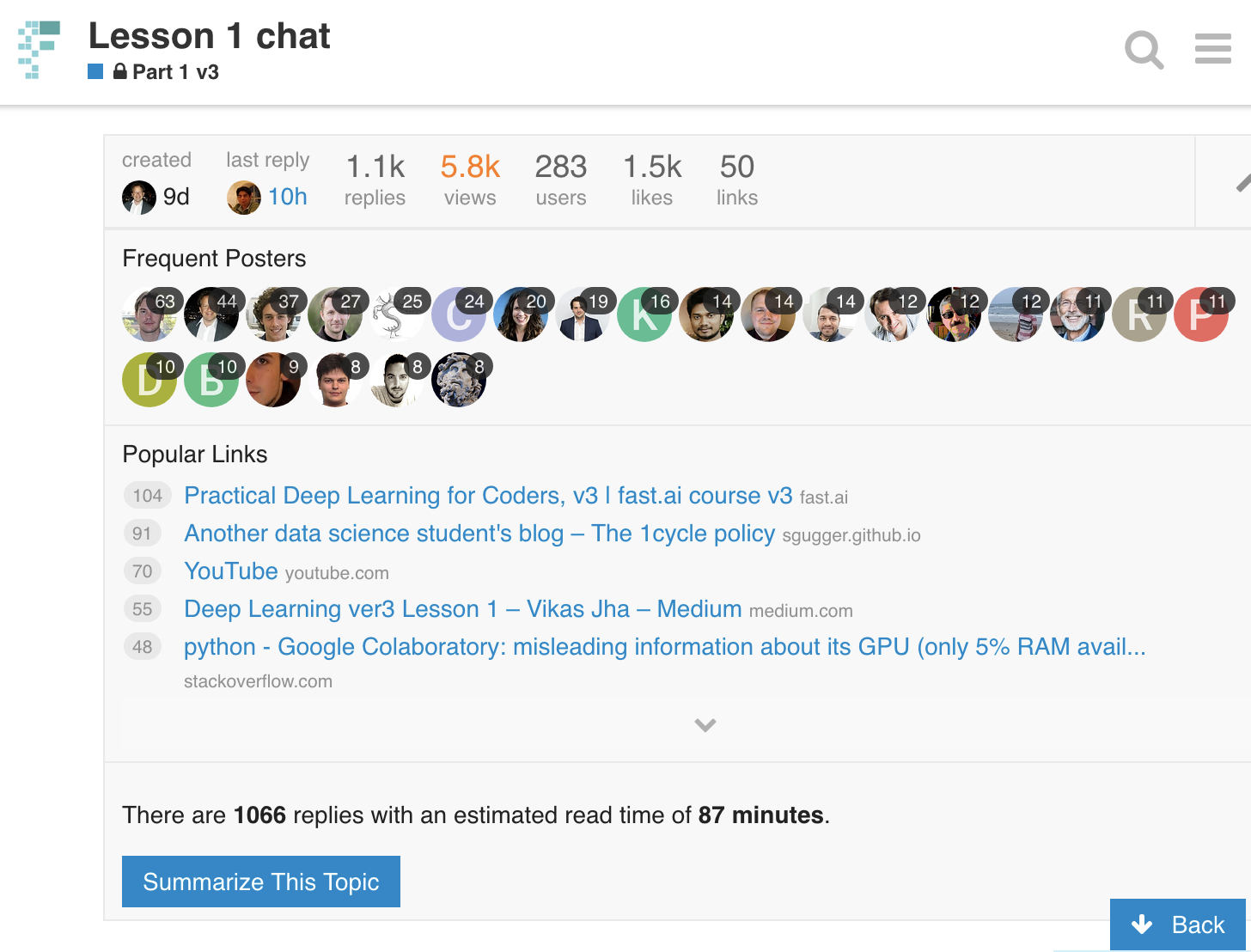
"Summarize This Topic" [2:32]
After just one week, the most popular thread has 1.1k replies which is intimidatingly large number. You shouldn't need to read all of it. What you should do is click "Summarize This Topic" and it will only show the most liked ones.
Returning to work [3:19]
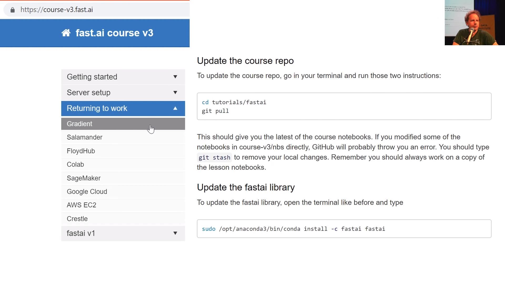
On the official course website, https://course-v3.fast.ai/ now has a "Returning to work" section which will show you (for each specific platform you use):
- How to make sure you have the latest notebooks
- How to make sure you have the latest fastai library
If things aren't working for you, if you get into some kind of messy situation, which we all do, just delete your instance and start again unless you've got mission-critical stuff there — it's the easiest way just to get out of a sticky situation.
What people have been doing this week [4:19]

- Figuring out who is talking — is it Ben Affleck or Joe Rogan
- Cleaning up WhatsApp downloaded images folder to get rid of memes
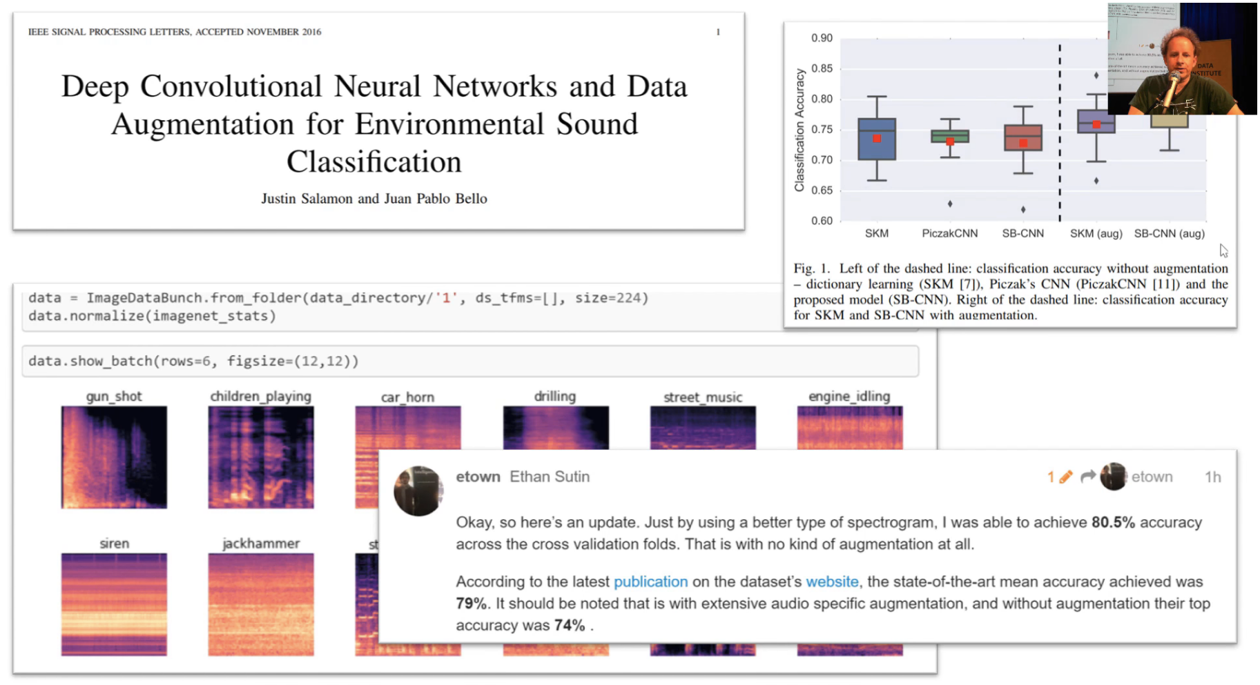
Deep Convolutional Neural Networks for Environmental Sound Classification
One of the really interesting projects was looking at the sound data that was used in this paper. In this paper, they were trying to figure out what kind of sound things were. They got a state of the art of nearly 80% accuracy. Ethan Sutin then tried using the lesson 1 techniques and got 80.5% accuracy, so I think this is pretty awesome. Best as we know, it's a new state of the art for this problem. Maybe somebody since has published something we haven't found it yet. So take all of these with a slight grain of salt, but I've mentioned them on Twitter and lots of people on Twitter follow me, so if anybody knew that there was a much better approach, I'm sure somebody would have said so.
[6:01]
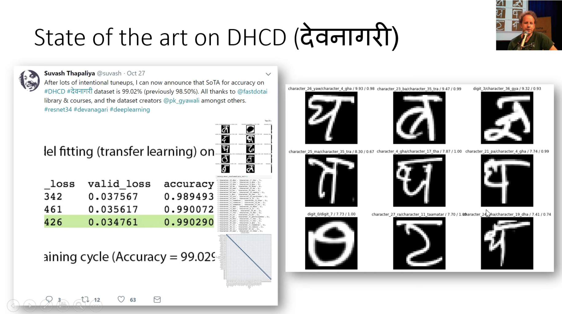
State of the art on Devanagari dataset/DHCD
Suvash has a new state of the art accuracy for Devanagari text recognition. I think he's got it even higher than this now. This is actually confirmed by the person on Twitter who created the dataset. I don't think he had any idea, he just posted here's a nice thing I did and this guy on Twitter said: "Oh, I made that dataset. Congratulations, you've got a new record." So that was pretty cool.
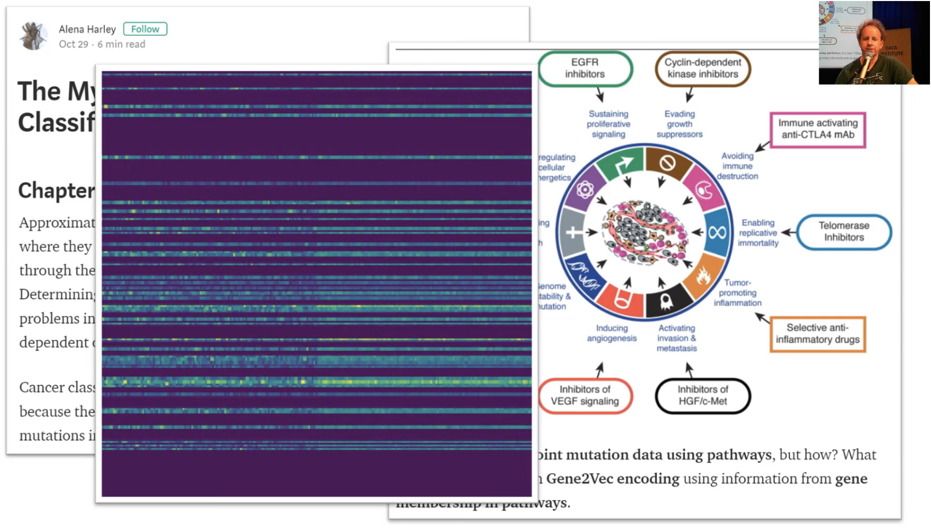
I really like this post from Alena Harley. She describes in quite a bit of detail about the issue of metastasizing cancers and the use of point mutations and why that's a challenging important problem. She's got some nice pictures describing what she wants to do with this and how she can go about turning this into pictures. This is the cool trick — it's the same with urning sounds into pictures and then using the lesson 1 approach. Here is turning point mutations into pictures and then using the lesson 1 approach. And it seems that she's got a new state of the art result by more than 30% beating the previous best. Somebody on Twitter who is a VP at a genomics analysis company looked at this as well and thought it looked to be a state of the art in this particular point mutation one as well. So that's pretty exciting.
When we talked about last week this idea that this simple process is something which can take you a long way, it really can. I will mention that something like this one in particular is using a lot of domain expertise, like figuring out that picture to create. I wouldn't know how to do that because I don't really know what a point mutation is, let alone how to create something that visually is meaningful that a CNN could recognize. But the actual deep learning side is actually pretty straight forward.
[8:07]
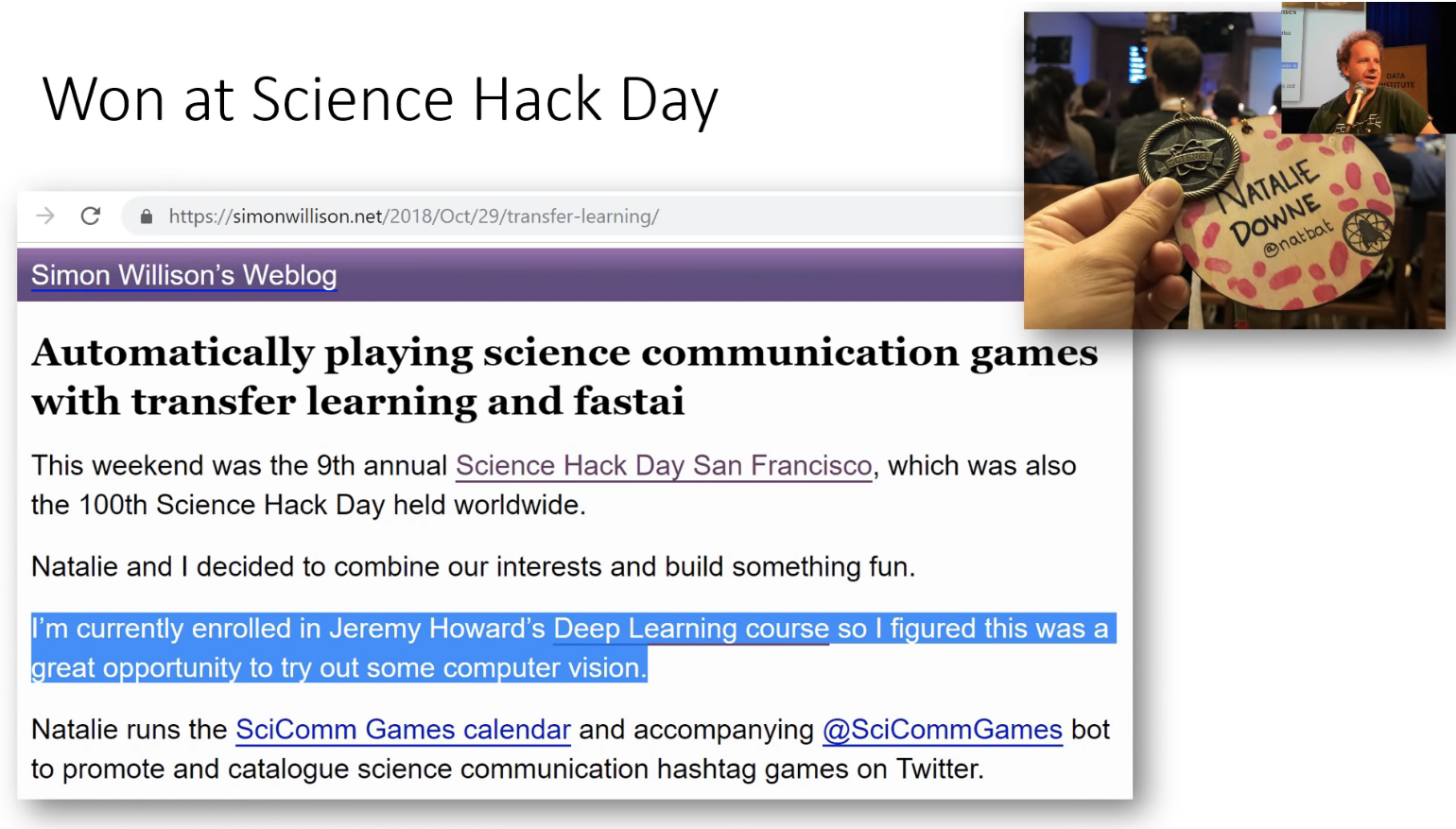
Another cool result from Simon Willison and Natalie Downe, they created a cougar or not web application over the weekend and won the Science Hack Day award in San Francisco. So I think that's pretty fantastic. So lots of examples of people doing really interesting work. Hopefully this will be inspiring to you to think well to think wow, this is cool that I can do this with what I've learned. It can also be intimidating to think like wow, these people are doing amazing things. But it's important to realize that as thousands of people are doing this course, I'm just picking out a few of really amazing ones. And in fact Simon is one of these very annoying people like Christine Payne who we talked about last week who seems to be good at everything he does. He created Django which is the world's most popular web frameworks, he founded a very successful startup, etc. One of those annoying people who tends to keep being good at things, now turns out he's good at deep learning as well. So that's fine. Simon can go on and win a hackathon on his first week of playing with deep learning. Maybe it'll take you two weeks to win your first hackathon. That's okay.
[9:22]
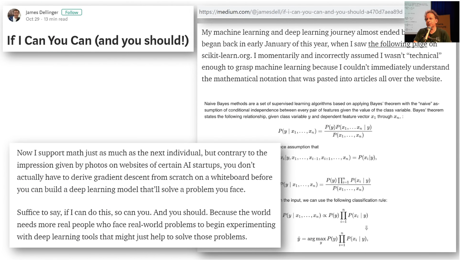
I think it's important to mention this because there was this really inspiring blog post this week from James Dellinger who talked about how he created a bird classifier using techniques from lesson 1. But what I really found interesting was at the end, he said he nearly didn't start on deep learning at all because he went through the scikit-learn website which is one of the most important libraries of Python and he saw this. And he described in this post how he was just like that's not something I can do. That's not something I understand. Then this kind of realization of like oh, I can do useful things without reading the Greek, so I thought that was really cool message.
[10:01]
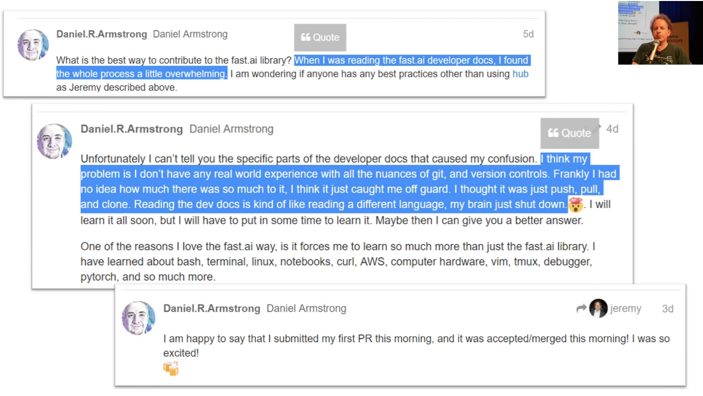
I really wanted to highlight Daniel Armstrong on the forum. I think really shows he's a great role model here. He was saying I want to contribute to the library and I looked at the docs and I just found it overwhelming. The next message, one day later, was I don't know what any of this is, I didn't know how much there is to it, caught me off guard, my brain shut down but I love the way it forces me to learn so much. And a day later, I just submitted my first pull request. So I think that's awesome. It's okay to feel intimidated. There's a lot. But just pick one piece and dig into it. Try and push a piece of code or a documentation update, or create a classifier or whatever.
[10:49]
So here's lots of cool classifiers people have built. It's been really inspiring.
- Trinidad and Tobago islanders versus masquerader classifier.
- A zucchini versus cucumber classifier.
- Dog and cat breed classifier from last week and actually doing some exploratory work to see what the main features were, and discovered that one was most hairy dog and naked cats. So there are interesting you can do with interpretation.
- Somebody else in the forum took that and did the same thing for anime to find that they had accidentally discovered an anime hair color classifier.
- We can now detect the new versus the old Panamanian buses.
- Henri Palacci discovered that he can recognize with 85% accuracy which of 110 countries a satellite image is of which is definitely got to be beyond human performance of just about anybody.
- Batik cloth classification with a hundred percent accuracy.
- Dave Luo did this interesting one. He actually went a little bit further using some techniques we'll be discussing in the next couple of courses to build something that can recognize complete/incomplete/foundation buildings and actually plot them on aerial satellite view.
So lots and lots of fascinating projects. So don't worry. It's only been one week. It doesn't mean everybody has to have had a project out yet. A lot of the folks who already have a project out have done a previous course, so they've got a bit of a head start. But we will see today how you can definitely create your own classifier this week.
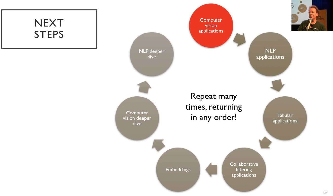
So from today, after we did a bit deeper into really how to make these computer vision classifiers and particular work well, we're then going to look at the same thing for text. We're then going to look at the same thing for tabular data. They are more like spreadsheets and databases. Then we're going to look at collaborative filtering (i.e. recommendation systems). That's going to take us into a topic called embeddings which is a key underlying platform behind these applications. That will take us back into more computer vision and then back into more NLP. So the idea here is that it turns out that it's much better for learning if you see things multiple times so rather than being like okay, that's computer vision, you won't see it again for the rest of the course, we're actually going to come back to the two key applications NLP and computer vision a few weeks apart. That's going to force your brain to realize oh, I have to remember this. It's not must something I can throw away.
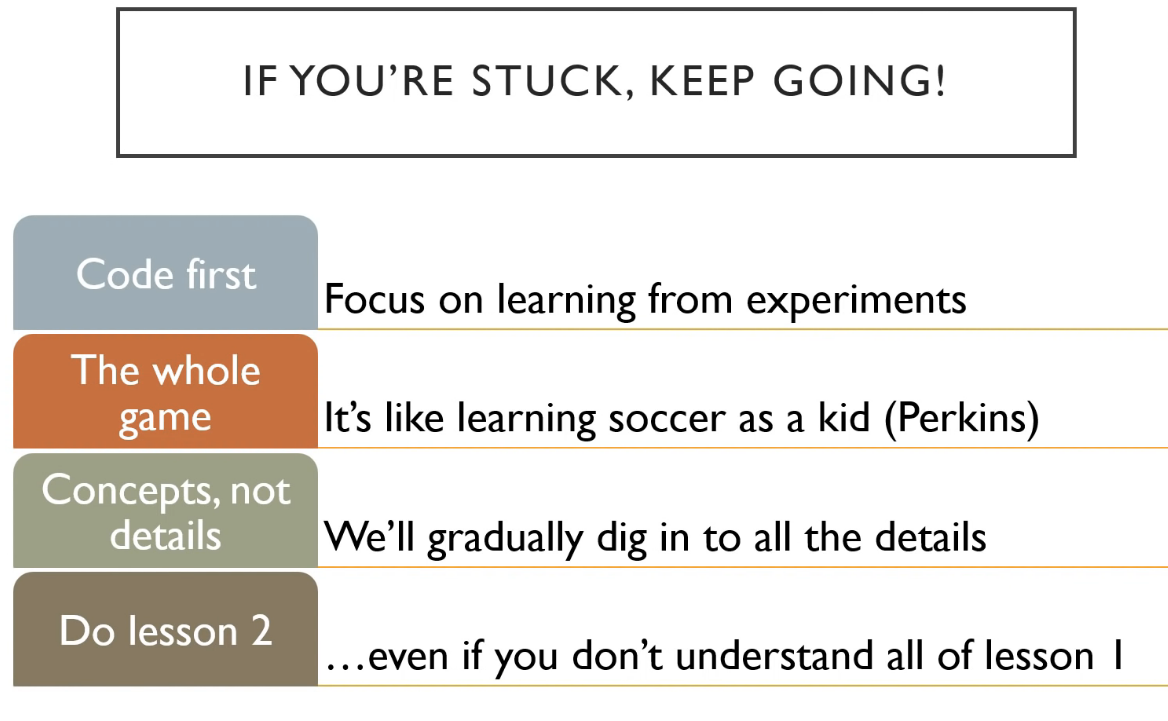
For people who have more of a hard sciences background in particular, a lot of folks find this hey, here's some code, type it in, start running it approach rather than here's lots of theory approach confusing and surprising and odd at first. So for those of you, I just wanted to remind you this basic tip which is keep going. You're not expected to remember everything yet. You're not expected to understand everything yet. You're not expected to know why everything works yet. You just want to be in a situation where you can enter the code and you can run it and you can get something happening and then you can start to experiment and you get a feel for what's going on. Then push on. Most of the people who have done the course and have gone on to be really successful watch the videos at least three times. So they kind of go through the whole lot and then go through it slowly the second time, then they go through it really slowly the third time. I consistently hear them say I get a lot more out of it each time I go through. So don't pause at lesson 1 and stop until you can continue.
This approach is based on a lot of academic research into learning theory. One guy in particular David Perkins from Harvard has this really great analogy. He is a researcher into learning theory. He describes this approach of whole game which is basically if you're teaching a kid to play soccer, you don't first of all teach them about how the friction between a ball and grass works and then teach them how to saw a soccer ball with their bare hands, and then teach them the mathematics of parabolas when you kick something in the air. No. You say, here's a ball. Let's watch some people playing soccer. Okay, now we'll play soccer and then gradually over the following years, learn more and more so that you can get better and better at it. So this is kind of what we're trying to get you to do is to play soccer which in our case is to type code and look at the inputs and look at the outputs.
Teddy bear detector using Google Images [16:21]
Let's dig into our first notebook which is called lesson2-download.ipynb. What we are going to do is we are going to see how to create your own classifier with your own images. It's going to be a lot like last week's pet detector but it will detect whatever you like. So to be like some of those examples we just saw. How would you create your own Panama bus detector from scratch. This is approach is inspired by Adrian Rosebrock who has a terrific website called PyiImageSearch and he has this nice explanation of "how to create a deep learning dataset using Google Images". So that was definitely an inspiration for some of the techniques we use here, so thank you to Adrian and you should definitely check out his site. It's full of lots of good resources.
We are going to try to create a teddy bear detector. And we're going to separate teddy bears from black bears, from grizzly bears. This is very important. I have a three year old daughter and she needs to know what she's dealing with. In our house, you would be surprised at the number of monsters, lions, and other terrifying threats that are around particularly around Halloween. So we always need to be on the lookout to make sure that the things we're about to cuddle is in fact a genuine teddy bear. So let's deal with that situation as best as we can.
Step 1: Get a list of URLs of each category of images
Our starting point is to find some pictures of teddy bears so we can learn what they look like. So I go to Google Images and I type in Teddy bear and I just scroll through until I find a goodly bunch of them. Okay, that looks like plenty of teddy bears to me.
Then I go back to the notebook and you can see it says "go to Google Images and search and scroll." The next thing we need to do is to get a list of all the URLs there. To do that, back in your google images, you hit CtrlShiftJ in Windows/Linux and CmdOptJ in Mac, and you paste the following into the window that appears:
urls = Array.from(document.querySelectorAll('.rg_di .rg_meta')).map(el=>JSON.parse(el.textContent).ou);
window.open('data:text/csv;charset=utf-8,' + escape(urls.join('\n')));
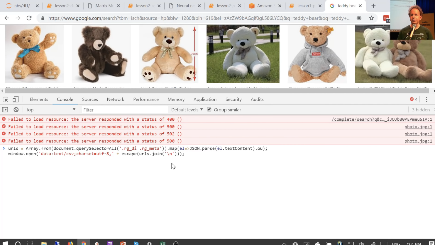
This is a Javascript console for those of you who haven't done any Javascript before. I hit enter and it downloads my file for me. So I would call this teddies.txt and press "Save". Okay, now I have a file containing URLs of teddies. Then I would repeat that process for black bears and for grizzly bears, and I put each one in a file with an appropriate name.
Step 2: Download images [19:39]
So step 2 is we now need to download those URLs to our server. Because remember when we're using Jupyter Notebook, it's not running on our computer. It's running on SageMaker or Crestle, or Google Cloud, etc. So to do that, we start running some Jupyter cells. Let's grab the fastai library:
from fastai import *
from fastai.vision import *
And let's start with black bears. So I click on this cell for black bears and I'll run it. So here, I've got three different cells doing the same thing but different information. This is one way I like to work with Jupyter notebook. It's something that a lot of people with more strict scientific background are horrified by. This is not reproducible research. I click on the black bear cell, and run it to create a folder called black and a file called urls_black.txt for my black bears. I skip the next two cells.
folder = 'black'
file = 'urls_black.txt'
folder = 'teddys'
file = 'urls_teddys.txt'
folder = 'grizzly'
file = 'urls_grizzly.txt'
Then I run this cell to create that folder.
path = Path('data/bears')
dest = path/folder
dest.mkdir(parents=True, exist_ok=True)
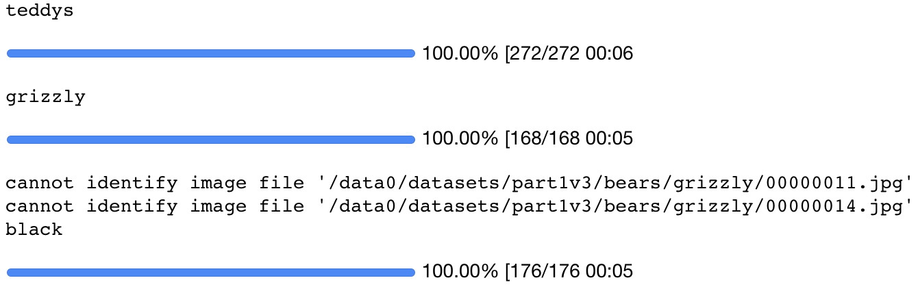
Then I go down to the next section and I run the next cell which is download images for black bears. So that's just going to download my black bears to that folder.
classes = ['teddys','grizzly','black']
download_images(path/file, dest, max_pics=200)
Now I go back and I click on 'teddys'. And I scroll back down and repeat the same thing. That way, I'm just going backwards and forwards to download each of the classes that I want. Very manual bur for me, I'm very iterative and very experimental, that work swell for me. If you are better at planning ahead than I am, you can write a proper loop or whatever and do it that way. But when you see my notebooks and see things that are kind of like configuration cells (i.e. doing the same thing in different places), this is a strong sign that I didn't run this in order. I clicked one place, went to another, ran that. For me, I'm experimentalist. I really like to experiment in my notebook, I treat it like a lab journal, I try things out and I see what happens. So this is how my notebooks end up looking.
It's a really controversial topic. For a lot of people, they feel this is "wrong" that you should only ever run things top to bottom. Everything you do should be reproducible. For me, I don't think that's the best way of using human creativity. I think human creativity is best inspired by trying things out and seeing what happens and fiddling around. You can see how you go. See what works for you.
So that will download the images to your server. It's going to use multiple processes to do so. One problem there is if something goes wrong, it's a bit hard to see what went wrong. So you can see in the next section, there's a commented out section that says max_workers=0. That will do it without spinning up a bunch of processes and will tell you the errors better. So if things aren't downloading, try using the second version.
# If you have problems download, try with `max_workers=0` to see exceptions:
# download_images(path/file, dest, max_pics=20, max_workers=0)
Step 3: Create ImageDataBunch [22:50]
The next thing that I found I needed to do was to remove the images that aren't actually images at all. This happens all the time. There's always a few images in every batch that are corrupted for whatever reason. Google image told us this URL had an image but it doesn't anymore. So we got this thing in the library called verify_images which will check all of the images in a path and will tell you if there's a problem. If you say delete=True, it will actually delete it for you. So that's a really nice easy way to end up with a clean dataset.
for c in classes:
    print(c)
    verify_images(path/c, delete=True, max_workers=8)
So at this point, I now have a bears folder containing a grizzly folder, teddys folder, and black folder. In other words, I have the basic structure we need to create an ImageDataBunch to start doing some deep learning. So let's go ahead and do that.
Now, very often, when you download a dataset from like Kaggle or from some academic dataset, there will often be folders called train, valid, and test containing the different datasets. In this case, we don't have a separate validation set because we just grabbed these images from Google search. But you still need a validation set, otherwise you don't know how well your model is going and we'll talk more about this in a moment.
Whenever you create a data bunch, if you don't have a separate training and validation set, then you can just say the training set is in the current folder (i.e. . because by default, it looks in a folder called train) and I want you to set aside 20% of the data, please. So this is going to create a validation set for you automatically and randomly. You'll see that whenever I create a validation set randomly, I always set my random seed to something fixed beforehand. This means that every time I run this code, I'll get the same validation set. In general, I'm not a fan of making my machine learning experiments reproducible (i.e. ensuring I get exactly the same results every time). The randomness is to me a really important part of finding out your is solution stable and it is going to work each time you run it. But what is important is that you always have the same validation set. Otherwise when you are trying to decide has this hyper parameter change improved my model but you've got a different set of data you are testing it on, then you don't know maybe that set of data just happens to be a bit easier. So that's why I always set the random seed here.
np.random.seed(42)
data = ImageDataBunch.from_folder(path, train=".", valid_pct=0.2,
        ds_tfms=get_transforms(), size=224, num_workers=4).normalize(imagenet_stats)
[25:37]
We've now got a data bunch, so you can look inside at the data.classes and you'll see these are the folders that we created. So it knows that the classes (by classes, we mean all the possible labels) are black bear, grizzly bear, or teddy bear.
data.classes
['black', 'grizzly', 'teddys']
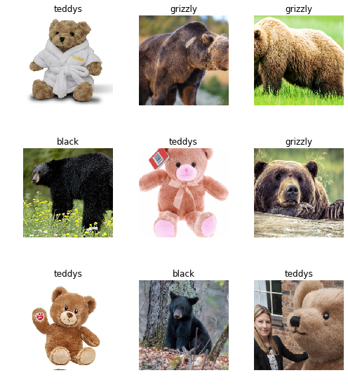
We can run show_batch and take a little look. And it tells us straight away that some of these are going to be a little bit tricky. Some of them are not photo, for instance. Some of them are cropped funny, if you ended up with a black bear standing on top of a grizzly bear, that might be tough.
data.show_batch(rows=3, figsize=(7,8))
You can kind of double check here. Remember, data.c is the attribute which the classifiers tell us how many possible labels there are. We'll learn about some other more specific meanings of c later. We can see how many things are now training set, how many things are in validation set. So we've got 473 training set, 141 validation set.
data.classes, data.c, len(data.train_ds), len(data.valid_ds)
(['black', 'grizzly', 'teddys'], 3, 473, 140)
Step 4: Training a model [26:49]
So at that point, we can go ahead and create our convolutional neural network using that data. I tend to default to using a resnet34, and let's print out the error rate each time.
learn = create_cnn(data, models.resnet34, metrics=error_rate)
Then run fit_one_cycle 4 times and see how we go. And we have a 2% error rate. So that's pretty good. Sometimes it's easy for me to recognize a black bear from a grizzly bear, but sometimes it's a bit tricky. This one seems to be doing pretty well.
learn.fit_one_cycle(4)
Total time: 00:54
epoch  train_loss  valid_loss  error_rate
1      0.710584    0.087024    0.021277    (00:14)
2      0.414239    0.045413    0.014184    (00:13)
3      0.306174    0.035602    0.014184    (00:13)
4      0.239355    0.035230    0.021277    (00:13)
After I make some progress with my model and things are looking good, I always like to save where I am up to to save me the 54 seconds of going back and doing it again.
learn.save('stage-1')
As per usual, we unfreeze the rest of our model. We are going to be learning more about what that means during the course.
learn.unfreeze()
Then we run the learning rate finder and plot it (it tells you exactly what to type). And we take a look.
learn.lr_find()
LR Finder complete, type {learner_name}.recorder.plot() to see the graph.
We are going to be learning about learning rates today, but for now, here's what you need to know. On the learning rate finder, what you are looking for is the strongest downward slope that's kind of sticking around for quite a while. It's something you are going to have to practice with and get a feel for﹣which bit works. So if you are not sure which, try both learning rates and see which one works better. I've been doing this for a while and I'm pretty sure this (between 10^-5 and 10^-3) looks like where it's really learning properly, so I will probably pick something back here for my learning rate [28:28].
learn.recorder.plot()
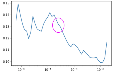
So you can see, I picked 3e-5 for my bottom learning rate. For my top learning rate, I normally pick 1e-4 or 3e-4, it's kind of like I don't really think about it too much. That's a rule of thumb﹣it always works pretty well. One of the things you'll realize is that most of these parameters don't actually matter that much in detail. If you just copy the numbers that I use each time, the vast majority of the time, it'll just work fine. And we'll see places where it doesn't today.
learn.fit_one_cycle(2, max_lr=slice(3e-5,3e-4))
Total time: 00:28
epoch  train_loss  valid_loss  error_rate
1      0.107059    0.056375    0.028369    (00:14)
2      0.070725    0.041957    0.014184    (00:13)
So we've got 1.4% error rate after doing another couple of epochs, so that's looking great. So we've downloaded some images from Google image search, created a classifier, and we've got 1.4% error rate, let's save it.
learn.save('stage-2')
Interpretation [29:38]
As per usual, we can use the ClassificationInterpretation class to have a look at what's going on.
learn.load('stage-2')
interp = ClassificationInterpretation.from_learner(learn)
interp.plot_confusion_matrix()
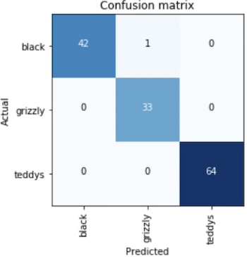
In this case, we made one mistake. There was one black bear classified as grizzly bear. So that's a really good step. We've come a long way. But possibly you could do even better if your dataset was less noisy. Maybe Google image search didn't give you exactly the right images all the time. So how do we fix that? We want to clean it up. So combining human expert with a computer learner is a really good idea. Very very few people publish on this or teach this, but to me, it's the most useful skill, particularly for you. Most of the people watching this are domain experts, not computer science experts, so this is where you can use your knowledge of point mutations in genomics or Panamanian buses or whatever. So let's see how that would work. What I'm going to do is, do you remember the plot top losses from last time where we saw the images which it was either the most wrong about or the least confident about. We are going to look at those and decide which of those are noisy. If you think about it, it's very unlikely that if there is a mislabeled data that it's going to be predicted correctly and with high confidence. That's really unlikely to happen. So we're going to focus on the ones which the model is saying either it's not confident of or it was confident of and it was wrong about. They are the things which might be mislabeled.
A big shout-out to the San Francisco fastai study group who created this new widget this week called the FileDeleter. Zach, Jason, and Francisco built this thing where we basically can take the top losses from that interpretation object we just created. There is not just plot_top-losses but there's also top_losses and top_losses returns two things: the losses of the things that were the worst and the indexes into the dataset of the things that were the worst. If you don't pass anything at all, it's going to actually return the entire dataset, but sorted so the first things will be the highest losses. Every dataset in fastai has x and y and the x contains the things that are used to, in this case, get the images. So this is the image file names and the y's will be the labels. So if we grab the indexes and pass them into the dataset's x, this is going to give us the file names of the dataset ordered by which ones had the highest loss (i.e. which ones it was either confident and wrong about or not confident about). So we can pass that to this new widget that they've created.
Just to clarify, this top_loss_paths contains all of the file names in our dataset. When I say "out dataset", this particular one is our validation dataset. So what this is going to do is it's going to clean up mislabeled images or images that shouldn't be there and we're going to remove them from a validation set so that our metrics will be more correct. You then need to rerun these two steps replacing valid_ds with train_ds to clean up your training set to get the noise out of that as well. So it's a good practice to do both. We'll talk about test sets later as well, if you also have a test set, you would then repeat the same thing.
from fastai.widgets import *

losses,idxs = interp.top_losses()
top_loss_paths = data.valid_ds.x[idxs]
fd = FileDeleter(file_paths=top_loss_paths)
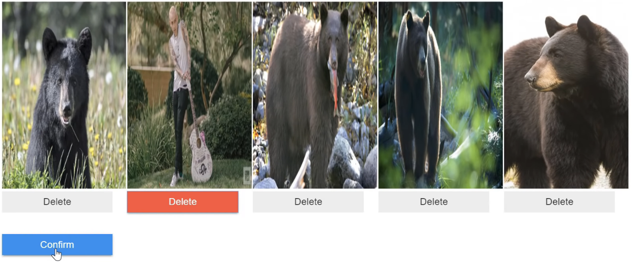
So we run FileDeleter passing in that sorted list of paths and so what pops up is basically the same thing as plot_top_losses. In other words, these are the ones which is either wrong about or least confident about. So not surprisingly, this one here (the second from left) does not appear to be a teddy bear, black bear, or grizzly bear. So this shouldn't be in our dataset. So what I do is I wack on the delete button, all the rest do look indeed like bears, so I can click confirm and it'll bring up another five.
What I tend to do when I do this is I'll keep going confirm until I get to a coupe of screen full of the things that all look okay and that suggests to me that I've got past the worst bits of the data. So that's it so now you can go back for the training set as well and retrain your model.
I'll just note here that what our San Francisco study group did here was that they actually built a little app inside Jupyter notebook which you might not have realized as possible. But not only is it possible, it's actually surprisingly straightforward. Just like everything else, you can hit double question mark to find out their secrets. So here is the source code.
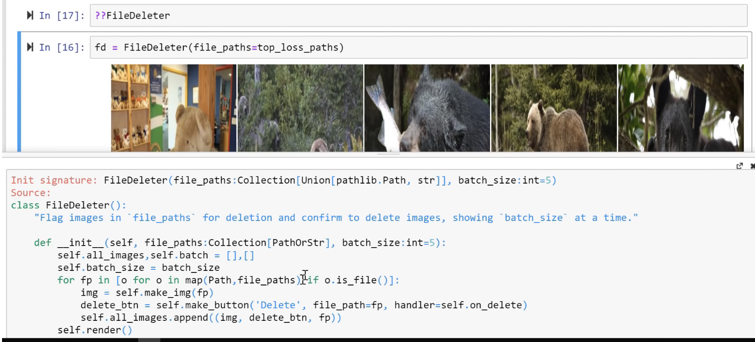
Really, if you've done any GUI programming before, it'll look incredibly normal. There's basically call backs for what happens when you click on a button where you just do standard Python things and to actually render it, you just use widgets and you can lay it out using standard boxes. So this idea of creating applications inside notebooks is really underused but it's super neat because it lets you create tools for your fellow practitioners or experimenters. And you could definitely envisage taking this a lot further. In fact, by the time you're watching this on the MOOC, you will probably find that there's a whole a lot more buttons here because we've already got a long list of to-do that we're going to add to this particular thing.
I'd love for you to have a think about, now that you know it's possible to write applications in your notebook, what are you going to write and if you google for "ipywidgets", you can learn about the little GUI framework to find out what kind of widgets you can create, what they look like, and how they work, and so forth. You'll find it's actually a pretty complete GUI programming environment you can play with. And this will all work nice with your models. It's not a great way to productionize an application because it is sitting inside a notebook. This is really for things which are going to help other practitioners or experimentalists. For productionizing things, you need to actually build a production web app which we will look at next.
Putting your model in production [37:36]
After you have cleaned up your noisy images, you can then retrain your model and hopefully you'll find it's a little bit more accurate. One thing you might be interested to discover when you do this is it actually doesn't matter most of the time very much. On the whole, these models are pretty good at dealing with moderate amounts of noisy data. The problem would occur is if your data was not randomly noisy but biased noisy. So I guess the main thing I'm saying is if you go through this process of cleaning up your data and then rerun your model and find it's .001% better, that's normal. It's fine. But it's still a good idea just to make sure that you don't have too much noise in your data in case it is biased.
At this point, we're ready to put our model in production and this is where I hear a lot of people ask me about which mega Google Facebook highly distributed serving system they should use and how do they use a thousand GPUs at the same time. For the vast majority of things you all do, you will want to actually run in production on a CPU, not a GPU. Why is that? Because GPU is good at doing lots of things at the same time, but unless you have a very busy website, it's pretty unlikely that you're going to have 64 images to classify at the same time to put into a batch into a GPU. And if you did, you've got to deal with all that queuing and running it all together, all of your users have to wait until that batch has got filled up and run﹣it's whole a lot of hassle. Then if you want to scale that, there's another whole lot of hassle. It's much easier if you just wrap one thing, throw it at a CPU to get it done, and comes back again. Yes, it's going to take maybe 10 or 20 times longer so maybe it'll take 0.2 seconds rather than 0.01 seconds. That's about the kind of times we are talking about. But it's so easy to scale. You can chuck it on any standard serving infrastructure. It's going to be cheap, and you can horizontally scale it really easily. So most people I know who are running apps that aren't at Google scale, based on deep learning are using CPUs. And the term we use is "inference". When you are not training a model but you've got a trained model and you're getting it to predict things, we call that inference. That's why we say here:
You probably want to use CPU for inference
At inference time, you've got your pre-trained model, you saved those weights, and how are you going to use them to create something like Simon Willison's cougar detector?
The first thing you're going to need to know is what were the classes that you trained with. You need to know not just what are they but what were the order. So you will actually need to serialize that or just type them in, or in some way make sure you've got exactly the same classes that you trained with.
data.classes
['black', 'grizzly', 'teddys']
If you don't have a GPU on your server, it will use the CPU automatically. If you have a GPU machine and you want to test using a CPU, you can just uncomment this line and that tells fastai that you want to use CPU by passing it back to PyTorch.
# fastai.defaults.device = torch.device('cpu')
[41:14]
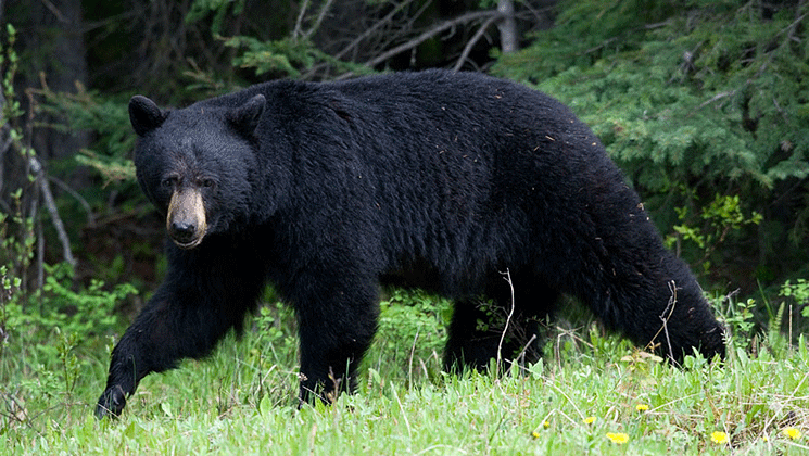
So here is an example. We don't have a cougar detector, we have a teddy bear detector. And my daughter Claire is about to decide whether to cuddle this friend. What she does is she takes daddy's deep learning model and she gets a picture of this and here is a picture that she's uploaded to the web app and here is a picture of the potentially cuddlesome object. We are going to store that in a variable called img , and open_image is how you open an image in fastai, funnily enough.
img = open_image(path/'black'/'00000021.jpg')
img
Here is that list of classes that we saved earlier. And as per usual, we created a data bunch, but this time, we're not going to create a data bunch from a folder full of images, we're going to create a special kind of data bunch which is one that's going to grab one single image at a time. So we're not actually passing it any data. The only reason we pass it a path is so that it knows where to load our model from. That's just the path that's the folder that the model is going to be in.
But what we need to do is that we need to pass it the same information that we trained with. So the same transforms, the same size, the same normalization. This is all stuff we'll learn more about. But just make sure it's the same stuff that you used before.
Now you've got a data bunch that actually doesn't have any data in it at all. It's just something that knows how to transform a new image in the same way that you trained with so that you can now do inference.
You can now create_cnn with this kind of fake data bunch and again, you would use exactly the same model that you trained with. You can now load in those saved weights. So this is the stuff that you only do once﹣just once when your web app is starting up. And it takes 0.1 of a second to run this code.
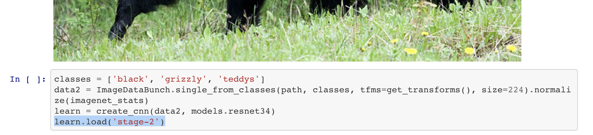
classes = ['black', 'grizzly', 'teddys']
data2 = ImageDataBunch.single_from_classes(path, classes, tfms=get_transforms(), size=224).normalize(imagenet_stats)
learn = create_cnn(data2, models.resnet34)
learn.load('stage-2')
Then you just go learn.predict(img) and it's lucky we did that because it's not a teddy bear. This is actually a black bear. So thankfully due to this excellent deep learning model, my daughter will avoid having a very embarrassing black bear cuddle incident.
pred_class,pred_idx,outputs = learn.predict(img)
pred_class
'black'
So what does this look like in production? I took Simon Willison's code, shamelessly stole it, made it probably a little bit worse, but basically it's going to look something like this. Simon used a really cool web app toolkit called Starlette. If you've ever used Flask, this will look extremely similar but it's kind of a more modern approach﹣by modern what I really mean is that you can use await which is basically means that you can wait for something that takes a while, such as grabbing some data, without using up a process. So for things like I want to get a prediction or I want to load up some data, it's really great to be able to use this modern Python 3 asynchronous stuff. So Starlette could come highly recommended for creating your web app.
You just create a route as per usual in the web app, in that you say this is async to ensure it doesn't steal the process while it's waiting for things.
You open your image you call learner.predict and you return that response. Then you can use Javascript client or whatever to show it. That's it. That's basically the main contents of your web app.
@app.route("/classify-url", methods=["GET"])
async def classify_url(request):
    bytes = await get_bytes(request.query_params["url"])
    img = open_image(BytesIO(bytes))
    _,_,losses = learner.predict(img)
    return JSONResponse({
        "predictions": sorted(
            zip(cat_learner.data.classes, map(float, losses)),
            key=lambda p: p[1],
            reverse=True
        )
    })
So give it a go this week. Even if you've never created a web application before, there's a lot of nice little tutorials online and kind of starter code, if in doubt, why don't you try Starlette. There's a free hosting that you can use, there's one called PythonAnywhere, for example. The one Simon has used, Zeit Now, it's something you can basically package it up as a Docker thing and shoot it off and it'll serve it up for you. So it doesn't even need to cost you any money and all these classifiers that you're creating, you can turn them into web application. I'll be really interested to see what you're able to make of that. That'll be really fun.
https://course-v3.fast.ai/deployment_zeit.html
Things that can go wrong [46:06]
I mentioned that most of the time, the kind of rules of thumb I've shown you will probably work. And if you look at the share your work thread, you'll find most of the time, people are posting things saying I downloaded these images, I tried this thing, they worked much better than I expected, well that's cool. Then like 1 out of 20 says I had a problem. So let's have a talk about what happens when you have a problem. This is where we start getting into a little bit of theory because in order to understand why we have these problems and how we fix them, it really helps to know a little bit about what's going on.
First of all, let's look at examples of some problems. The problems basically will be either:
- Your learning rate is too high or low
- Your number of epochs is too high or low
So we are going to learn about what those mean and why they matter. But first of all, because we are experimentalists, let's try them.
Learning rate (LR) too high
So let's grow with our teddy bear detector and let's make our learning rate really high. The default learning rate is 0.003 that works most of the time. So what if we try a learning rate of 0.5. That's huge. What happens? Our validation loss gets pretty darn high. Remember, this is something that's normally something underneath 1. So if you see your validation loss do that, before we even learn what validation loss is, just know this, if it does that, your learning rate is too high. That's all you need to know. Make it lower. Doesn't matter how many epochs you do. If this happens, there's no way to undo this. You have to go back and create your neural net again and fit from scratch with a lower learning rate.
learn = create_cnn(data, models.resnet34, metrics=error_rate)
learn.fit_one_cycle(1, max_lr=0.5)
Total time: 00:13
epoch  train_loss  valid_loss  error_rate
1      12.220007   1144188288.000000  0.765957    (00:13)
Learning rate (LR) too low [48:02]
What if we used a learning rate not of 0.003 but 1e-5 (0.00001)?
learn = create_cnn(data, models.resnet34, metrics=error_rate)
This is just copied and pasted what happened when we trained before with a default learning rate:
Total time: 00:57
epoch  train_loss  valid_loss  error_rate
1      1.030236    0.179226    0.028369    (00:14)
2      0.561508    0.055464    0.014184    (00:13)
3      0.396103    0.053801    0.014184    (00:13)
4      0.316883    0.050197    0.021277    (00:15)
And within one epoch, we were down to a 2 or 3% error rate.
With this really low learning rate, our error rate does get better but very very slowly.
learn.fit_one_cycle(5, max_lr=1e-5)
Total time: 01:07
epoch  train_loss  valid_loss  error_rate
1      1.349151    1.062807    0.609929    (00:13)
2      1.373262    1.045115    0.546099    (00:13)
3      1.346169    1.006288    0.468085    (00:13)
4      1.334486    0.978713    0.453901    (00:13)
5      1.320978    0.978108    0.446809    (00:13)
And you can plot it. So learn.recorder is an object which is going to keep track of lots of things happening while you train. You can call plot_losses to plot out the validation and training loss. And you can just see them gradually going down so slow. If you see that happening, then you have a learning rate which is too small. So bump it by 10 or bump it up by 100 and try again. The other thing you see if your learning rate is too small is that your training loss will be higher than your validation loss. You never want a model where your training loss is higher than your validation loss. That always means you haven't fitted enough which means either your learning rate is too low or your number of epochs is too low. So if you have a model like that, train it some more or train it with a higher learning rate.
learn.recorder.plot_losses()
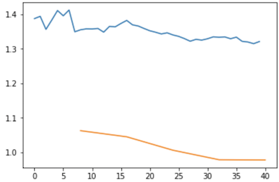
As well as taking a really long time, it's getting too many looks at each image, so may overfit.
Too few epochs [49:42]
What if we train for just one epoch? Our error rate is certainly better than random, 5%. But look at this, the difference between training loss and validation loss ﹣ a training loss is much higher than the validation loss. So too few epochs and too lower learning rate look very similar. So you can just try running more epochs and if it's taking forever, you can try a higher learning rate. If you try a higher learning rate and the loss goes off to 100,000 million, then put it back to where it was and try a few more epochs. That's the balance. That's all you care about 99% of the time. And this is only the 1 in 20 times that the defaults don't work for you.
learn = create_cnn(data, models.resnet34, metrics=error_rate, pretrained=False)
learn.fit_one_cycle(1)
Total time: 00:14
epoch  train_loss  valid_loss  error_rate
1      0.602823    0.119616    0.049645    (00:14)
Too many epochs [50:30]
Too many epochs create something called "overfitting". If you train for too long as we're going to learn about it, it will learn to recognize your particular teddy bears but not teddy bears in general. Here is the thing. Despite what you may have heard, it's very hard to overfit with deep learning. So we were trying today to show you an example of overfitting and I turned off everything. I turned off all the data augmentation, dropout, and weight decay. I tried to make it overfit as much as I can. I trained it on a small-ish learning rate, I trained it for a really long time. And maybe I started to get it to overfit. Maybe.
So the only thing that tells you that you're overfitting is that the error rate improves for a while and then starts getting worse again. You will see a lot of people, even people that claim to understand machine learning, tell you that if your training loss is lower than your validation loss, then you are overfitting. As you will learn today in more detail and during the rest of course, that is absolutely not true.
Any model that is trained correctly will always have train loss lower than validation loss.
That is not a sign of overfitting. That is not a sign you've done something wrong. That is a sign you have done something right. The sign that you're overfitting is that your error starts getting worse, because that's what you care about. You want your model to have a low error. So as long as you're training and your model error is improving, you're not overfitting. How could you be?
np.random.seed(42)
data = ImageDataBunch.from_folder(path, train=".", valid_pct=0.9, bs=32,
        ds_tfms=get_transforms(do_flip=False, max_rotate=0, max_zoom=1, max_lighting=0, max_warp=0
                              ),size=224, num_workers=4).normalize(imagenet_stats)
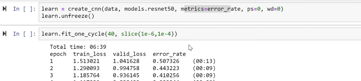
learn = create_cnn(data, models.resnet50, metrics=error_rate, ps=0, wd=0)
learn.unfreeze()
learn.fit_one_cycle(40, slice(1e-6,1e-4))
Total time: 06:39
epoch  train_loss  valid_loss  error_rate
1      1.513021    1.041628    0.507326    (00:13)
2      1.290093    0.994758    0.443223    (00:09)
3      1.185764    0.936145    0.410256    (00:09)
4      1.117229    0.838402    0.322344    (00:09)
5      1.022635    0.734872    0.252747    (00:09)
6      0.951374    0.627288    0.192308    (00:10)
7      0.916111    0.558621    0.184982    (00:09)
8      0.839068    0.503755    0.177656    (00:09)
9      0.749610    0.433475    0.144689    (00:09)
10     0.678583    0.367560    0.124542    (00:09)
11     0.615280    0.327029    0.100733    (00:10)
12     0.558776    0.298989    0.095238    (00:09)
13     0.518109    0.266998    0.084249    (00:09)
14     0.476290    0.257858    0.084249    (00:09)
15     0.436865    0.227299    0.067766    (00:09)
16     0.457189    0.236593    0.078755    (00:10)
17     0.420905    0.240185    0.080586    (00:10)
18     0.395686    0.255465    0.082418    (00:09)
19     0.373232    0.263469    0.080586    (00:09)
20     0.348988    0.258300    0.080586    (00:10)
21     0.324616    0.261346    0.080586    (00:09)
22     0.311310    0.236431    0.071429    (00:09)
23     0.328342    0.245841    0.069597    (00:10)
24     0.306411    0.235111    0.064103    (00:10)
25     0.289134    0.227465    0.069597    (00:09)
26     0.284814    0.226022    0.064103    (00:09)
27     0.268398    0.222791    0.067766    (00:09)
28     0.255431    0.227751    0.073260    (00:10)
29     0.240742    0.235949    0.071429    (00:09)
30     0.227140    0.225221    0.075092    (00:09)
31     0.213877    0.214789    0.069597    (00:09)
32     0.201631    0.209382    0.062271    (00:10)
33     0.189988    0.210684    0.065934    (00:09)
34     0.181293    0.214666    0.073260    (00:09)
35     0.184095    0.222575    0.073260    (00:09)
36     0.194615    0.229198    0.076923    (00:10)
37     0.186165    0.218206    0.075092    (00:09)
38     0.176623    0.207198    0.062271    (00:10)
39     0.166854    0.207256    0.065934    (00:10)
40     0.162692    0.206044    0.062271    (00:09)
[52:23]
So they are the main four things that can go wrong. There are some other details that we will learn about during the rest of this course but honestly if you stopped listening now (please don't, that would be embarrassing) and you're just like okay I'm going to go and download images, I'm going to create CNNs with resnet34 or resnet50, I'm going to make sure that my learning rate and number of epochs is okay and then I'm going to chuck them up in a Starlette web API, most of the time you are done. At least for computer vision. Hopefully you will stick around because you want to learn about NLP, collaborative filtering, tabular data, and segmentation, and stuff like that as well.
[53:10]
Let's now understand what's actually going on. What does "loss" mean? What does "epoch" mean? What does "learning rate" mean? Because for you to really understand these ideas, you need to know what's going on. So we are going to go all the way to the other side. Rather than creating a state of the art cougar detector, we're going to go back and create the simplest possible linear model. So we're going to actually seeing a little bit of math. But don't be turned off. It's okay. We're going to do a little bit of math but it's going to be totally fine. Even if math is not your thing. Because the first thing we're going to realize is that when we see a picture like this number eight:
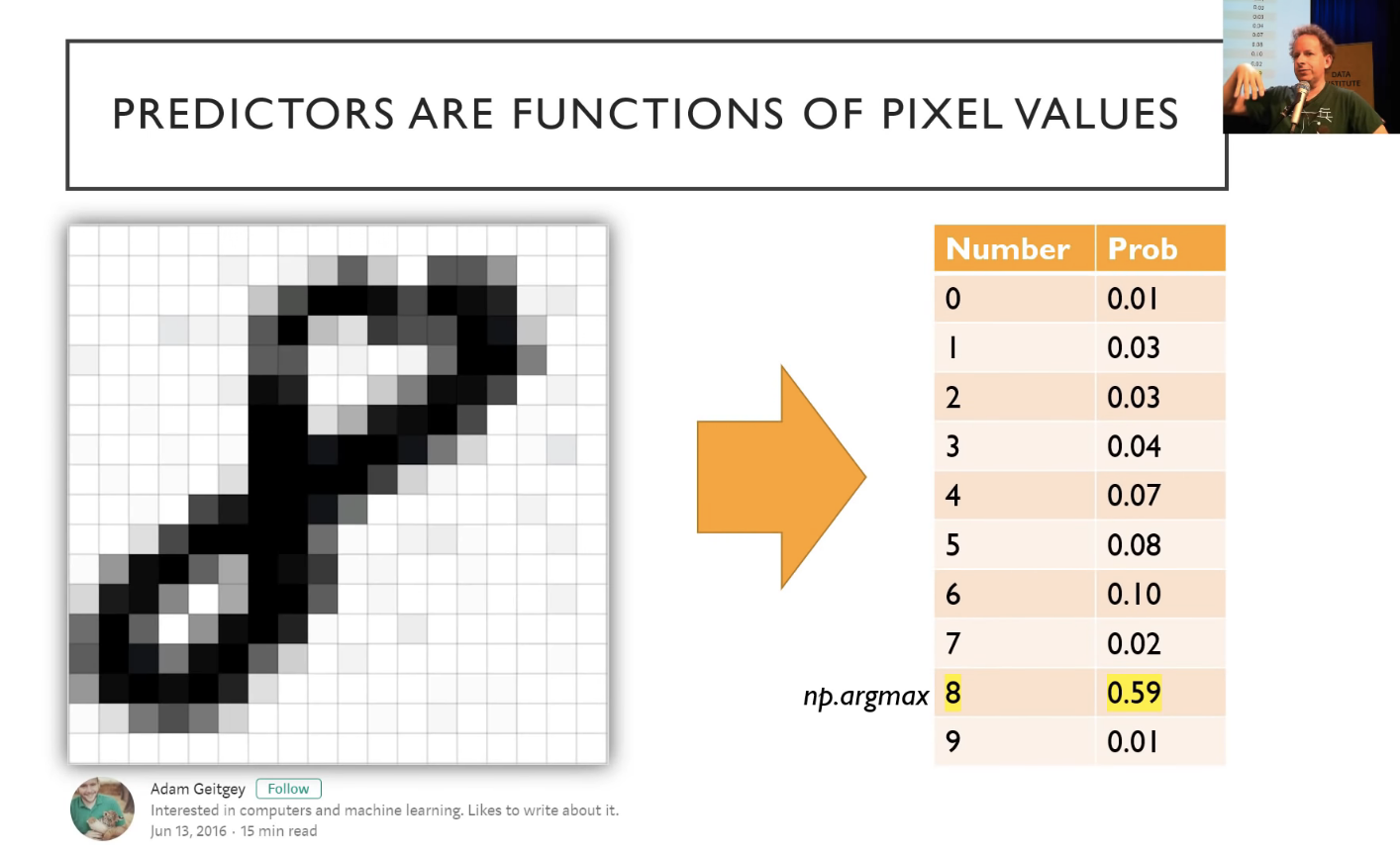
It's actually just a bunch of numbers. For this grayscale one, it's a matrix of numbers. If it was a color image, it would have a third dimension. So when you add an extra dimension, we call it a tensor rather than a matrix. It would be a 3D tensor of numbers ﹣ red, green, and blue.
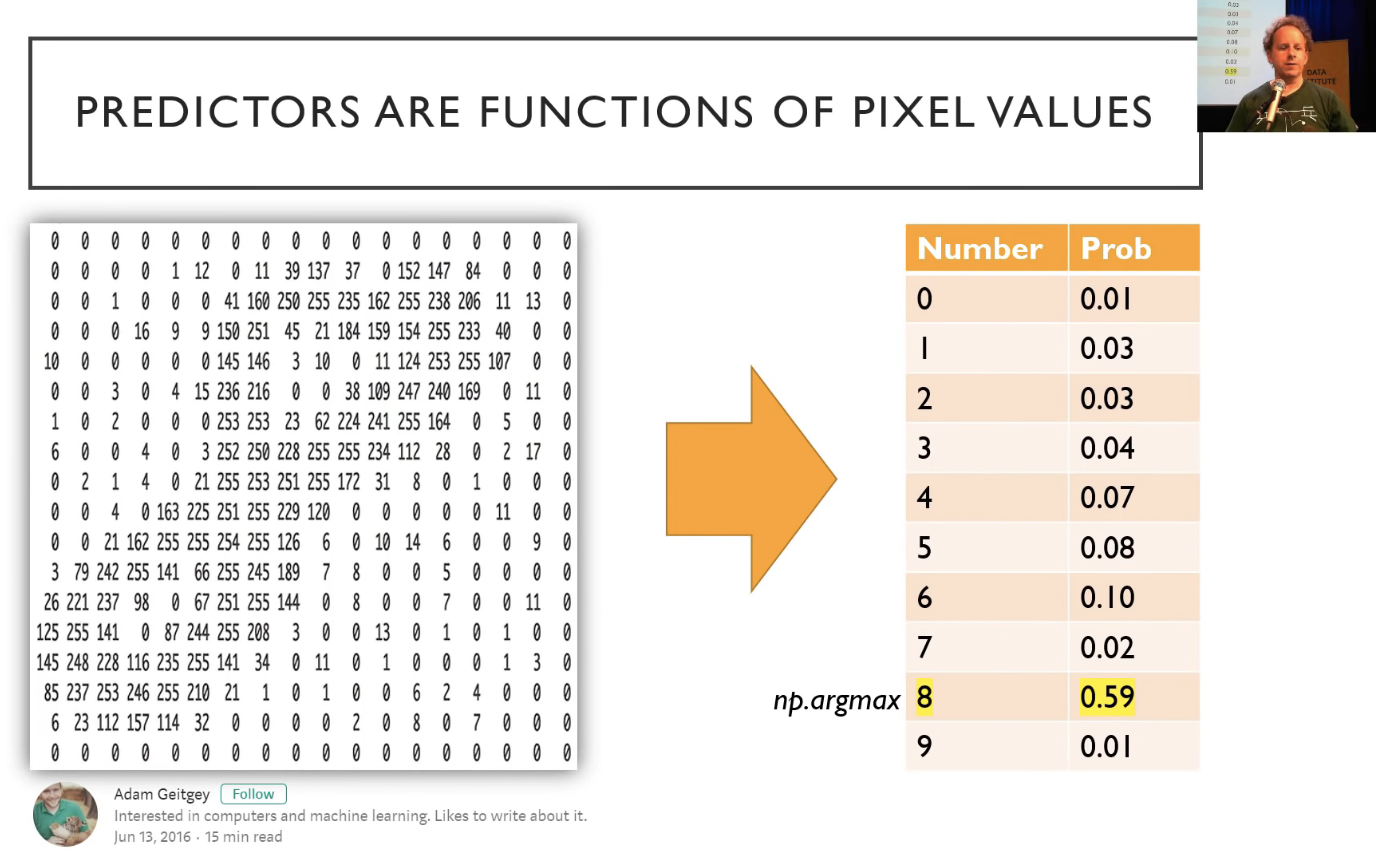
So when we created that teddy bear detector, what we actually did was we created a mathematical function that took the numbers from the images of the teddy bears and a mathematical function converted those numbers into, in our case, three numbers: a number for the probability that it's a teddy, a probability that it's a grizzly, and the probability that it's a black bear. In this case, there's some hypothetical function that's taking the pixel representing a handwritten digit and returning ten numbers: the probability for each possible outcome (i.e. the numbers from zero to nine).
So what you'll often see in our code and other deep learning code is that you'll find this bunch of probabilities and then you'll find a function called max or argmax attached to it. What that function is doing is, it's saying find the highest number (i.e. probability) and tell me what the index is. So np.argmax or torch.argmax of the above array would return the index 8.
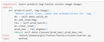
In fact, let's try it. We know that the function to predict something is called learn.predict. So we can chuck two question marks before or after it to get the source code.
![]()
And here it is. pred_max = res.argmax(). Then what is the class? We just pass that into the classes array. So you should find that the source code in the fastai library can both strengthen your understanding of the concepts and make sure that you know what's going on and really help you here.
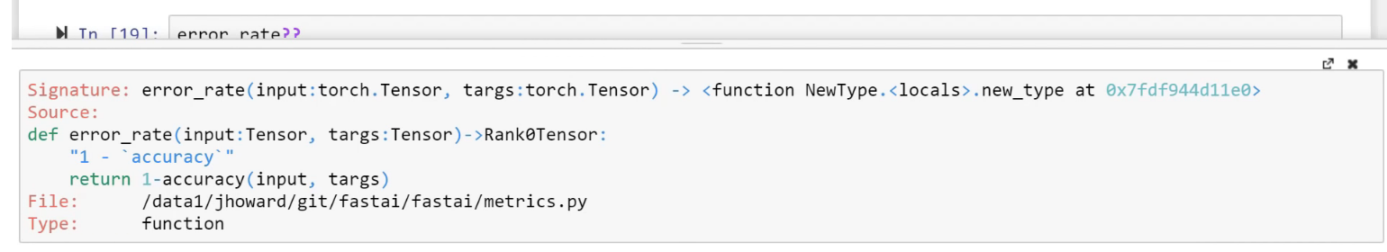
Question: Can we have a definition of the error rate being discussed and how it is calculated? I assume it's cross validation error [56:38].
Sure. So one way to answer the question of how is error rate calculated would be to type error_rate?? and look at the source code, and it's 1 - accuracy.
So then a question might be what is accuracy:
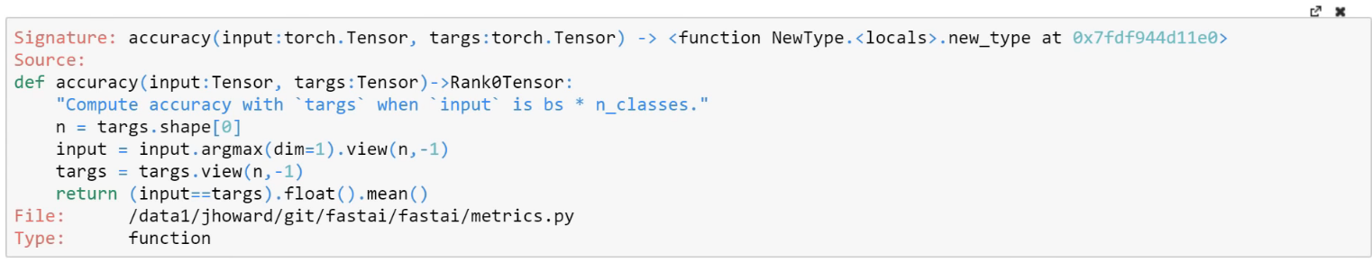
It is argmax. So we now know that means find out which particular thing it is, and then look at how often that equals the target (i.e. the actual value) and take the mean. So that's basically what it is. So then the question is, okay, what does that being applied to and always in fastai, metrics (i.e. the things that we pass in) are always going to be applied to the validation set. Any time you put a metric here, it'll be applied to the validation set because that's your best practice:
That's what you always want to do is make sure that you're checking your performance on data that your model hasn't seen, and we'll be learning more about the validation set shortly.
Remember, you can also type doc if the source code is not what you want which might well not be, you actually want the documentation, that will both give you a summary of the types in and out of the function and a link to the full documentation where you can find out all about how metrics work and what other metrics there are and so forth. Generally speaking, you'll also find links to more information where, for example, you will find complete run through and sample code showing you how to use all these things. So don't forget that the doc function is your friend. Also both in the doc function and in documentation, you'll see a source link. This is like ?? but what the source link does is it takes you into the exact line of code in Github. So you can see exactly how that's iplemented and what else is around it. So lots of good stuff there.
Question: Why were you using 3e for your learning rates earlier? With 3e-5 and 3e-4 [59:11]?
We found that 3e-3 is just a really good default learning rate. It works most of the time for your initial fine-tuning before you unfreeze. And then, I tend to kind of just multiply from there. So then the next stage, I will pick 10 times lower than that for the second part of the slice, and whatever the LR finder found for the first part of the slice. The second part of the slice doesn't come from the LR finder. It's just a rule of thumb which is 10 times less than your first part which defaults to 3e-3, and then the first part of the slice is what comes out of the LR finder. We'll be learning a lot more about these learning rate details both today and in the coming lessons. But for now, all you need to remember is that your basic approach looks like this:
learn.fit_one_cycle- Some number of epochs, I often pick 4
- Some learning rate which defaults to 3e-3. I'll just type it up fully so you can see.
- Then we do that for a bit and then we unfreeze it.
- Then we learn some more and so this is a bit where I just take whatever I did last time and divide it by 10. Then I also write like that (
slice) then I have to put one more number in here and that's the number I get from the learning rate finder﹣a bit where it's got the strongest slope.
learn.fit_one_cycle(4, 3e-3)
learn.unfreeze()
learn.fit_one_cycle(4, slice(xxx, 3e-4))
So that's kind of don't have to think about it, don't really have to know what's going on rule of thumb that works most of the time. But let's now dig in and actually understand it more completely.
Digging in and looking at the math [1:01:17]
We're going to create this mathematical function that takes the numbers that represent the pixels and spits out probabilities for each possible class.

By the way, a lot of the stuff that we're using here, we are stealing from other people who are awesome and so we're putting their details here. So please check out their work because they've got great work that we are highlighting in our course. I really like this idea of this little animated gif of the numbers, so thank you to Adam Geitgey for creating that.
[1:02:05]
Let's look and see how we create one of these functions, and let's start with the simplest functions I know:
That's a line where
- a: gradient of the line
- b: the intercept of the line
Hopefully when we said that you need to know high school math to do this course, these are the things we are assuming that you remember. If we do mention some math thing which I am assuming you remember and you don't remember it, don't freak out. It happens to all of us. Khan Academy is actually terrific. It's not just for school kids. Go to Khan Academy, find the concept you need a refresher on, and he explains things really well. So strongly recommend checking that out. Remember, I'm just a philosophy student, so all the time I'm trying to either remind myself about something or I never learnt something. So we have the whole internet to teach us these things.
I'm going to re-write this slightly:
So let's just replace with a
_, just give it a different name. So there's another way of saying the same thing. Then another way of saying that would be if I could multiply
by the number 1.
This still is the same thing. Now at this point, I'm actually going to say let's not put the number 1 there, but put an here and
here:
So far, this is pretty early high school math. This is multiplying by 1 which I think we can handle. So this and are equivalent with a bit of renaming. Now in machine learning, we don't just have one equation, we've got lots. So if we've got some data that represents the temperature versus the number of ice creams sold, then we have lots of dots.
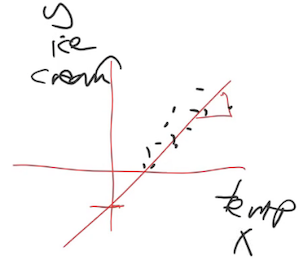
So each one of those dots, we might hypothesize is based on this formula (). And basically there's lots of values of y and lots of values of x so we can stick little
here:
The way we do that is a lot like numpy indexing, but rather things in square brackets, we put them down here in the subscript in our equation:
So this is now saying there's actually lots of these different 's based on lots of different
and
but notice there is still one of each of these (
,
). They called the coefficients or the parameters. So this is our linear equation and we are still going to say that every
is equal to 1. Why did I do it that way? Because I want to do linear algebra? Why do I want to do in linear algebra? One reason is because Rachel teaches the world's best linear algebra course, so if you're interested, check it out. So it's a good opportunity for me to throw in a pitch for this which we make no money but never mind. But more to the point right now, it's going to make life much easier. Because I hate writing loops, I hate writing code, I just want the computer to do everything for me. And anytime you see this little i subscripts, that sounds like you're going to have to do loops and all kind of stuff. But what you might remember from school is that when you've got two things being multiplied together, two things being multiplied together, then they get added up, that's called a "dot product". If you do that for lots and lots of different numbers i, then that's called a matrix product. So in fact, this whole thing can be written like this:
Rather than lots of different 's, we can say there's one vector called
which is equal to one matrix called
times one vector called
. At this point, I know a lot of you don't remember that. That's fine. We have a picture to show you:
Andre Staltz created this fantastic called http://matrixmultiplication.xyz/ and here we have a matrix by a vector, and we are going to do a matrix vector product.
That is what matrix vector multiplication does. In other words, it's just except his version is much less messy.
Question: When generating new image dataset, how do you know how many images are enough? What are ways to measure "enough"? [1:08:35]
Great question. Another possible problem you have is you don't have enough data. How do you know if you don't have enough data? Because you found a good learning rate (i.e. if you make it higher than it goes off into massive losses; if you make it lower, it goes really slowly) and then you train for such a long time that your error starts getting worse. So you know that you trained for long enough. And you're still not happy with the accuracy﹣it's not good enough for the teddy bear cuddling level of safety you want. So if that happens, there's a number of things you can do and we'll learn pretty much all of them during this course but one of the easiest one is get more data. If you get more data, then you can train for longer, get a higher accuracy, lower error rate, without overfitting.
Unfortunately there is no shortcut. I wish there was. I wish there's some way to know ahead of time how much data you need. But I will say this﹣most of the time, you need less data than you think. So organizations very commonly spend too much time gathering data, getting more data than it turned out they actually needed. So get a small amount first and see how you go.
Question: What do you do if you have unbalanced classes such as 200 grizzly and 50 teddy? [1:10:00]
Nothing. Try it. It works. A lot of people ask this question about how do I deal with unbalanced data. I've done lots of analysis with unbalanced data over the last couple of years and I just can't make it not work. It always works. There's actually a paper that said if you want to get it slightly better then the best thing to do is to take that uncommon class and just make a few copies of it. That's called "oversampling" but I haven't found a situation in practice where I needed to do that. I've found it always just works fine, for me.
Question: Once you unfreeze and retrain with one cycle again, if your training loss is still higher than your validation loss (likely underfitting), do you retrain it unfrozen again (which will technically be more than one cycle) or you redo everything with longer epoch per the cycle? [1:10:47]
You guys asked me that last week. My answer is still the same. I don't know. Either is fine. If you do another cycle, then it'll maybe generalize a little bit better. If you start again, do twice as long, it's kind of annoying, depends how patient you are. It won't make much difference. For me personally, I normally just train a few more cycles. But it doesn't make much difference most of the time.
Question: Question about this code example:
classes = ['black', 'grizzly', 'teddys']
data2 = ImageDataBunch.single_from_classes(path, classes, tfms=get_transforms(), size=224).normalize(imagenet_stats)
learn = create_cnn(data2, models.resnet34)
learn.load('stage-2')
This requires models.resnet34 which I find surprising: I had assumed that the model created by .save(...) (which is about 85MB on disk) would be able to run without also needing a copy of resnet34. [1:11:37]
We're going to be learning all about this shortly. There is no "copy of ResNet34", ResNet34 is what we call "architecture"﹣it's a functional form. Just like is a linear functional form. It doesn't take up any room, it doesn't contain anything, it's just a function. ResNet34 is just a function. I think the confusion here is that we often use a pre-trained neural net that's been learnt on ImageNet. In this case, we don't need to use a pre-trained neural net. Actually, to avoid that even getting created, you can actually pass
pretrained=False:

That'll ensure that nothing even gets loaded which will save you another 0.2 seconds, I guess. But we'll be learning a lot more about this. So don't worry if this is a bit unclear. The basic idea is models.resnet34 above is basically the equivalent of saying is it a line or is it a quadratic or is it a reciprocal﹣this is just a function. This is a ResNet34 function. It's a mathematical function. It doesn't take any storage, it doesn't have any numbers, it doesn't have to be loaded as opposed to a pre-trained model. When we did it at the inference time, the thing that took space is this bit:
Which is where we load our parameters. It is basically saying, as we are about find out, what are the values of and
﹣ we have to store these numbers. But for ResNet34, you don't just store 2 numbers, you store a few million or few tens of millions of numbers.
[1:14:13]
So why did we all this? It's because I wanted to be able to write it out like this: and the reason I wanted to be able to like this is that we can now do that in PyTorch with no loops, single line of code, and it's also going to run faster.
PyTorch really doesn't like loops
It really wants you to send it a whole equation to do all at once. Which means, you really want to try and specify things in these kind of linear algebra ways. So let's go and take a look because what we're going to try and do then is we're going to try and take this (we're going to call this an architecture). It's the world's tiniest neural network. It's got two parameters
and
. We are going to try and fit this architecture to some data.
SGD [1:15:06]
So let's jump into a notebook and generate some dots, and see if we can get it to fit a line somehow. And the "somehow" is going to be using something called SGD. What is SGD? Well, there's two types of SGD. The first one is where I said in lesson 1 "hey you should all try building these models and try and come up with something cool" and you guys all experimented and found really good stuff. So that's where the S would be Student. That would be Student Gradient Descent. So that's version one of SGD.
Version two of SGD which is what I'm going to talk about today is where we are going to have a computer try lots of things and try and come up with a really good function and that would be called Stochastic Gradient Descent. The other one that you hear a lot on Twitter is Stochastic Grad student Descent.
Linear Regression problem [1:16:08]
We are going to jump into lesson2-sgd.ipynb. We are going to go bottom-up rather than top-down. We are going to create the simplest possible model we can which is going to be a linear model. And the first thing we need is we need some data. So we are going to generate some data. The data we're going to generate looks like this:

So x-axis might represent temperature, y-axis might represent number of ice creams we sell, or something like that. But we're just going to create some synthetic data that we know is following a line. As we build this, we're actually going to learn a little bit about PyTorch as well.
%matplotlib inline
from fastai import *
n=100
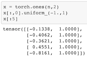
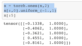
x = torch.ones(n,2)
x[:,0].uniform_(-1.,1)
x[:5]
tensor([[-0.1338,  1.0000],
        [-0.4062,  1.0000],
        [-0.3621,  1.0000],
        [ 0.4551,  1.0000],
        [-0.8161,  1.0000]])
Basically the way we're going to generate this data is by creating some coefficients. will be 3 and
will be 2. We are going to create a column of numbers for our
's and a whole bunch of 1's.
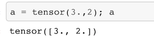
a = tensor(3.,2); a
tensor([3., 2.])
And then we're going to do this x@a. What is x@a? x@a in Python means a matrix product between x and a. And it actually is even more general than that. It can be a vector vector product, a matrix vector product, a vector matrix product, or a matrix matrix product. Then actually in PyTorch, specifically, it can mean even more general things where we get into higher rank tensors which we will learn all about very soon. But this is basically the key thing that's going to go on in all of our deep learning. The vast majority of the time, our computers are going to be basically doing this﹣multiplying numbers together and adding them up which is the surprisingly useful thing to do.
y = x@a + torch.rand(n)
[1:17:57]
So we basically are going to generate some data by creating a line and then we're going to add some random numbers to it. But let's go back and see how we created x and a. I mentioned that we've basically got these two coefficients 3 and 2. And you'll see that we've wrapped it in this function called tensor. You might have heard this word "tensor" before. It's one of these words that sounds scary and apparently if you're a physicist, it actually is scary. But in the world of deep learning, it's actually not scary at all. "tensor" means array, but specifically it's an array of a regular shape. So it's not an array where row 1 has two things, row 3 has three things, and row 4 has one thing, what you call a "jagged array". That's not a tensor. A tensor is any array which has a rectangular or cube or whatever ﹣ a shape where every row is the same length and every column is the same length. The following are all tensors:
- 4 by 3 matrix
- A vector of length 4
- A 3D array of length 3 by 4 by 6
That's all tensor is. We have these all the time. For example, an image is a 3 dimensional tensor. It's got number of rows by number of columns by number of channels (normally red, green, blue). So for example, VGA picture could be 640 by 480 by 3 or actually we do things backwards so when people talk about images, they normally go width by height, but when we talk mathematically, we always go a number of rows by number of columns, so it would actually be 480 by 640 by 3 that will catch you out. We don't say dimensions, though, with tensors. We use one of two words, we either say rank or axis. Rank specifically means how many axes are there, how many dimensions are there. So an image is generally a rank 3 tensor. What we created here is a rank 1 tensor (also known as a vector). But in math, people come up with very different words for slightly different concepts. Why is a one dimensional array a vector and a two dimensional array is a matrix, and a three dimensional array doesn't have a name. It doesn't make any sense. With computers, we try to have some simple consistent naming conventions. They are all called tensors﹣rank 1 tensor, rank 2 tensor, rank 3 tensor. You can certainly have a rank 4 tensor. If you've got 64 images, then that would be a rank 4 tensor of 64 by 480 by 640 by 3. So tensors are very simple. They just mean arrays.
In PyTorch, you say tensor and you pass in some numbers, and you get back, which in this case just a list, a vector. This then represents our coefficients: the slope and the intercept of our line.
Because we are not actually going to have a special case of , instead, we are going to say there's always this second
value which is always 1
You can see it here, always 1 which allows us just to do a simple matrix vector product:
So that's . Then we wanted to generate this
array of data. We're going to put random numbers in the first column and a whole bunch of 1's in the second column. To do that, we say to PyTorch that we want to create a rank 2 tensor of
n by 2. Since we passed in a total of 2 things, we get a rank 2 tensor. The number of rows will be n and the number of columns will be 2. In there, every single thing in it will be a 1﹣that's what torch.ones means.
[1:22:45]
Then this is really important. You can index into that just like you can index into a list in Python. But you can put a colon anywhere and a colon means every single value on that axis/dimension. This here x[:,0] means every single row of column 0. So x[:,0].uniform_(-1.,1) is every row of column 0, I want you to grab a uniform random numbers.
Here is another very important concept in PyTorch. Anytime you've got a function that ends with an underscore, it means don't return to me that uniform random number, but replace whatever this is being called on with the result of this function. So this x[:,0].uniform_(-1.,1) takes column 0 and replaces it with a uniform random number between -1 and 1. So there's a lot to unpack there.
But the good news is these two lines of code and x@a which we are coming to cover 95% of what you need to know about PyTorch.
- How to create an array
- How to change things in an array
- How to do matrix operations on an array
So there's a lot to unpack, but these small number of concepts are incredibly powerful. So I can now print out the first five rows. [:5] is a standard Python slicing syntax to say the first 5 rows. So here are the first 5 rows, 2 columns looking like﹣my random numbers and my 1's.
Now I can do a matrix product of that x by my a, add in some random numbers to add a bit of noise.
y = x@a + torch.rand(n)
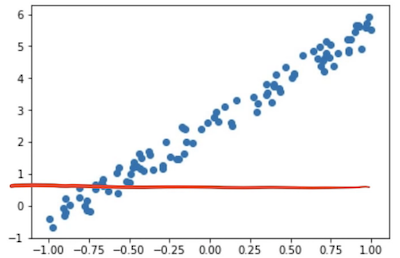
Then I can do a scatter plot. I'm not really interested in my scatter plot in this column of ones. They are just there to make my linear function more convenient. So I'm just going to plot my zero index column against my y's.
plt.scatter(x[:,0], y);
plt is what we universally use to refer to the plotting library, matplotlib. That's what most people use for most of their plotting in scientific Python. It's certainly a library you'll want to get familiar with because being able to plot things is really important. There are lots of other plotting packages. Lots of the other packages are better at certain things than matplotlib, but matplotlib can do everything reasonably well. Sometimes it's a little awkward, but for me, I do pretty much everything in matplotlib because there is really nothing it can't do even though some libraries can do other things a little bit better or prettier. But it's really powerful so once you know matplotlib, you can do everything. So here, I'm asking matplotlib to give me a scatterplot with my x's against my y's. So this is my dummy data representing temperature and ice cream sales.
Now what we're going to do is, we are going to pretend we were given this data and we don't know that the values of our coefficients are 3 and 2. So we're going to pretend that we never knew that and we have to figure them out. How would we figure them out? How would we draw a line to fit this data and why would that even be interesting? Well, we're going to look at more about why it's interesting in just a moment. But the basic idea is:
If we can find a way to find those two parameters to fit that line to those 100 points, we can also fit these arbitrary functions that convert from pixel values to probabilities.
It will turn out that this techniques that we're going to learn to find these two numbers works equally well for the 50 million numbers in ResNet34. So we're actually going to use an almost identical approach. This is the bit that I found in previous classes people have the most trouble digesting. I often find, even after week 4 or week 5, people will come up to me and say:
Student: I don't get it. How do we actually train these models?
Jeremy: It's SGD. It's that thing we saw in the notebook with the 2 numbers.
Student: yeah, but... but we are fitting a neural network.
Jeremy: I know and we can't print the 50 million numbers anymore, but it's literally identically doing the same thing.
The reason this is hard to digest is that the human brain has a lot of trouble conceptualizing of what an equation with 50 million numbers looks like and can do. So for now, you'll have to take my word for it. It can do things like recognize teddy bears. All these functions turn out to be very powerful. We're going to learn about how to make them extra powerful. But for now, this thing we're going to learn to fit these two numbers is the same thing that we've just been using to fit 50 million numbers.
Loss function [1:28:36]
We want to find what PyTorch calls parameters, or in statistics, you'll often hear it called coefficient (i.e. these values of and
). We want to find these parameters such that the line that they create minimizes the error between that line and the points. In other words, if the
and
we came up with resulted in this line:
Then we'd look and we'd see how far away is that line from each point. That's quite a long way. So maybe there was some other and
which resulted in the gray line. And they would say how far away is each of those points. And then eventually we come up with the yellow line. In this case, each of those is actually very close.
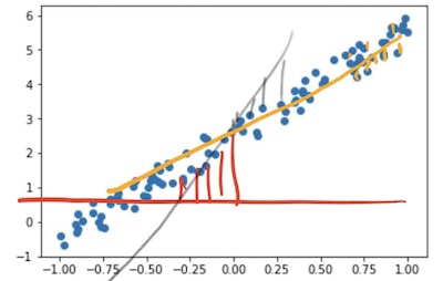
So you can see how in each case we can say how far away is the line at each spot away from its point, and then we can take the average of all those. That's called the loss. That is the value of our loss. So you need a mathematical function that can basically say how far away is this line from those points.
For this kind of problem which is called a regression problem (a problem where your dependent variable is continuous, so rather than being grizzlies or teddies, it's some number between -1 and 6), the most common loss function is called mean squared error which pretty much everybody calls MSE. You may also see RMSE which is root mean squared error. The mean squared error is a loss which is the difference between some predictions that you made which is like the value of the line and the actual number of ice cream sales. In the mathematics of this, people normally refer to the actual as and the prediction, they normally call it
(y hat).
When writing something like mean squared error equation, there is no point writing "ice cream" and "temperature" because we want it to apply to anything. So we tend to use these mathematical placeholders.
So the value of mean squared error is simply the difference between those two (y_hat-y) squared. Then we can take the mean because both y_hat and y are rank 1 tensors, so we subtract one vector from another vector, it does something called "element-wise arithmetic" in other words, it subtracts each one from each other, so we end up with a vector of differences. Then if we take the square of that, it squares everything in that vector. So then we can take the mean of that to find the average square of the differences between the actuals and the predictions.
def mse(y_hat, y): return ((y_hat-y)**2).mean()
If you're more comfortable with mathematical notation, what we just wrote was:
One of the things I'll note here is, I don't think ((y_hat-y)**2).mean() is more complicated or unwieldy than but the benefit of the code is you can experiment with it. Once you've defined it, you can use it, you can send things into it, get stuff out of it, and see how it works. So for me, most of the time, I prefer to explain things with code rather than with math. Because they are the same, just different notations. But one of the notations is executable. It's something you can experiment with. And the other is abstract. That's why I'm generally going to show code.
So the good news is, if you're a coder with not much of a math background, actually you do have a math background. Because code is math. If you've got more of a math background and less of a code background, then actually a lot of the stuff that you learned from math is going to translate directly into code and now you can start to experiment with your math.
[1:34:03]
mse is a loss function. This is something that tells us how good our line is. Now we have to come up with what is the line that fits through here. Remember, we are going to pretend we don't know. So what you actually have to do is you have to guess. You actually have to come up with a guess what are the values of and
. So let's say we guess that
and
are -1 and 1.
a = tensor(-1.,1)
Here is how you create that tensor and I wanted to write it this way because you'll see this all the time. Written out fully, it would be tensor(-1.0, 1.0). We can't write it without the point because tensor(-1, 1) is now an int, not a floating point. So that's going to spit the dummy (Australian for "behave in a bad-tempered or petulant way") if you try to do calculations with that in neural nets.
I'm far too lazy to type .0 every time. Python knows perfectly well that if you added . next to any of these numbers, then the whole thing is now floats. So that's why you'll often see it written this way, particularly by lazy people like me.
So a is a tensor. You can see it's floating-point. You see, even PyTorch is lazy. They just put a dot. They don't bother with a zero.

But if you want to actually see exactly what it is, you can write .type() and you can see it's a FloatTensor:
So now we can calculate our predictions with this random guess. x@a a matrix product of x and a. And we can now calculate the mean squared error of our predictions and their actuals, and that's our loss. So for this regression, our loss is 0.9.
y_hat = x@a
mse(y_hat, y)
tensor(8.8945)
So we can now plot a scatter plot of x against y and we can plot the scatter plot of x against y_hat. And there they are.
plt.scatter(x[:,0],y)
plt.scatter(x[:,0],y_hat);

So that is not great﹣not surprising. It's just a guess. So SGD or gradient descent more generally and anybody who's done engineering or probably computer science at school would have done plenty of this like Newton's method, etc at university. If you didn't, don't worry. We're going to learn it now.
It's basically about taking this guess and trying to make it a little bit better. How do we make it a little better? Well, there are only two numbers and the two numbers are the intercept of the orange line and the gradient of the orange line. So what we are going to do with gradient descent is we're going to simply say:
- What if we changed those two numbers a little bit?
- What if we made the intercept a little bit higher or a little bit lower?
- What if we made the gradient a little bit more positive or a little bit more negative?
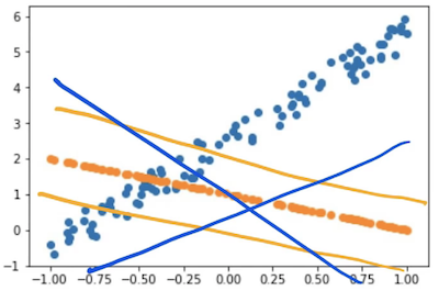
There are 4 possibilities and then we can calculate the loss for each of those 4 possibilities and see what works. Did lifting it up or down make it better? Did tilting it more positive or more negative make it better? And then all we do is we say, okay, whichever one of those made it better, that's what we're going to do. That's it.
But here is the cool thing for those of you that remember calculus. You don't actually have to move it up and down, and round about. You can actually calculate the derivative. The derivative is the thing that tells you would moving it up or down make it better, or would rotating it this way or that way make it better. The good news is if you didn't do calculus or you don't remember calculus, I just told you everything you need to know about it. It tells you how changing one thing changes the function. That's what the derivative is, kind of, not quite strictly speaking, but close enough, also called the gradient. The gradient or the derivative tells you how changing up or down would change our MSE, how changing
up or down would change our MSE, and this does it more quickly than actually moving it up and down.
In school, unfortunately, they forced us to sit there and calculate these derivatives by hand. We have computers. Computers can do that for us. We are not going to calculate them by hand.
a = nn.Parameter(a); a
Parameter containing:
tensor([-1.,  1.], requires_grad=True)
Instead, we're doing to call .grad. On our computer, that will calculate the gradient for us.
def update():
    y_hat = x@a
    loss = mse(y, y_hat)
    if t % 10 == 0: print(loss)
    loss.backward()
    with torch.no_grad():
        a.sub_(lr * a.grad)
        a.grad.zero_()
So here is what we're going to do. We are going to create a loop. We're going to loop through 100 times, and we're going to call a function called update. That function is going to:
- Calculate
y_hat(i.e. our prediction) - Calculate loss (i.e. our mean squared error)
- From time to time, it will print that out so we can see how we're going
- Calculate the gradient. In PyTorch, calculating the gradient is done by using a method called
backward. Mean squared error was just a simple standard mathematical function. PyTorch keeps track of how it was calculated and lets us calculate the derivative. So if you do a mathematical operation on a tensor in PyTorch, you can callbackwardto calculate the derivative and the derivative gets stuck inside an attribute called.grad. - Take my coefficients and I'm going to subtract from them my gradient (
sub_). There is an underscore there because that's going to do it in-place. It's going to actually update those coefficientsato subtract the gradients from them. Why do we subtract? Because the gradient tells us if I move the whole thing downwards, the loss goes up. If I move the whole thing upwards, the loss goes down. So I want to do the opposite of the thing that makes it go up. We want our loss to be small. That's why we subtract. lris our learning rate. All it is is the thing that we multiply by the gradient. Why is there anylrat all? Let me show you why.
Why is there any LR at all? [1:41:31]
Let's take a really simple example, a quadratic. And let's say your algorithm's job was to find where that quadratic was at its lowest point. How could it do this? Just like what we're doing now, the starting point would be just to pick some x value at random. Then find out what the value of y is. That's the starting point. Then it can calculate the gradient and the gradient is simply the slope, but it tells you moving in which direction is make you go down. So the gradient tells you, you have to go this way.
If the gradient was really big, you might jump left a very long way, so you might jump all the way over to here. If you jumped over there, then that's actually not going to be very helpful because it's worse. We jumped too far so we don't want to jump too far.
Maybe we should just jump a little bit. That is actually a little bit closer. So then we'll just do another little jump. See what the gradient is and do another little jump, and repeat.
In other words, we find our gradient to tell us what direction to go and if we have to go a long way or not too far. But then we multiply it by some number less than 1 so we don't jump too far.
Hopefully at this point, this might be reminding you of something which is what happened when our learning rate was too high.
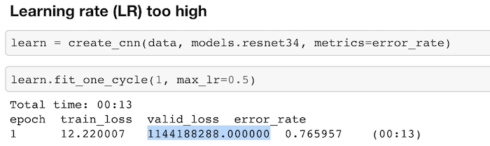
Do you see why that happened now? Our learning rate was too high meant that we jumped all the way past the right answer further than we started with, and it got worse, and worse, and worse. So that's what a learning rate too high does.
On the other hand, if our learning rate is too low, then you just take tiny little steps and so eventually you're going to get there, but you are doing lots and lots of calculations along the way. So you really want to find something where it's either big enough steps like stairs or a little bit of back and forth. You want something that gets in there quickly but not so quickly it jumps out and diverges, not so slowly that it takes lots of steps. That's why we need a good learning rate and that's all it does.
So if you look inside the source code of any deep learning library, you'll find this:
a.sub_(lr * a.grad)
You will find something that says "coefficients ﹣ learning rate times gradient". And we will learn about some easy but important optimization we can do to make this go faster.
That's about it. There's a couple of other little minor issues that we don't need to talk about now: one involving zeroing out the gradient and other involving making sure that you turn gradient calculation off when you do the SGD update. If you are interested, we can discuss them on the forum or you can do our introduction to machine learning course which covers all the mechanics of this in more detail.
Training loop [1:45:43]
If we run update 100 times printing out the loss from time to time, you can see it starts at 8.9, and it goes down.
lr = 1e-1
for t in range(100): update()
tensor(8.8945, grad_fn=<MeanBackward1>)
tensor(1.6115, grad_fn=<MeanBackward1>)
tensor(0.5759, grad_fn=<MeanBackward1>)
tensor(0.2435, grad_fn=<MeanBackward1>)
tensor(0.1356, grad_fn=<MeanBackward1>)
tensor(0.1006, grad_fn=<MeanBackward1>)
tensor(0.0892, grad_fn=<MeanBackward1>)
tensor(0.0855, grad_fn=<MeanBackward1>)
tensor(0.0843, grad_fn=<MeanBackward1>)
tensor(0.0839, grad_fn=<MeanBackward1>)
So you can then print out scatterplots and there it is.
plt.scatter(x[:,0],y)
plt.scatter(x[:,0],x@a);
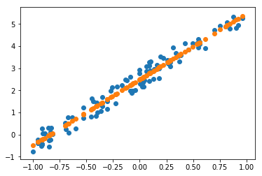
That's it! Believe it or not, that's gradient descent. So we just need to start with a function that's a bit more complex than x@a but as long as we have a function that can represent things like if this is a teddy bear, we now have a way to fit it.
Animate it! [1:46:20]
Let's now take a look at this as an animation. This is one of the nice things that you can do with matplotlib. You can take any plot and turn it into an animation. So you can now actually see it updating each step.
from matplotlib import animation, rc
rc('animation', html='html5')
You may need to uncomment the following to install the necessary plugin the first time you run this: (after you run following commands, make sure to restart the kernal for this notebook) If you are running in Colab, the installs are not needed; just change the cell above to be ... html='jshtml' instead of ... html='html5'
#! sudo add-apt-repository -y ppa:mc3man/trusty-media
#! sudo apt-get update -y
#! sudo apt-get install -y ffmpeg
#! sudo apt-get install -y frei0r-plugins
Let's see what we did here. We simply said, as before, create a scatter plot, but then rather than having a loop, we used matplotlib's FuncAnimation to call 100 times this animate function. And this function just calls that update we created earlier then update the y data in our line. Repeat that 100 times, waiting 20 milliseconds after each one.
a = nn.Parameter(tensor(-1.,1))

fig = plt.figure()
plt.scatter(x[:,0], y, c='orange')
line, = plt.plot(x[:,0], x@a)
plt.close()

def animate(i):
    update()
    line.set_ydata(x@a)
    return line,

animation.FuncAnimation(fig, animate, np.arange(0, 100), interval=20)
You might think visualizing your algorithms with animations is something amazing and complex thing to do, but actually now you know it's 11 lines of code. So I think it's pretty darn cool.
That is SGD visualized and we can't visualize as conveniently what updating 50 million parameters in a ResNet-34 looks like but basically doing the same thing. So studying these simple version is actually a great way to get an intuition. So you should try running this notebook with a really big learning rate, with a really small learning rate, and see what this animation looks like, and try to get a feel for it. Maybe you can even try a 3D plot. I haven't tried that yet, but I'm sure it would work fine.
Mini-batches [1:48:08]
The only difference between stochastic gradient descent and this is something called mini-batches. You'll see, what we did here was we calculated the value of the loss on the whole dataset on every iteration. But if your dataset is 1.5 million images in ImageNet, that's going to be really slow. Just to do a single update of your parameters, you've got to calculate the loss on 1.5 million images. You wouldn't want to do that. So what we do is we grab 64 images or so at a time at random, and we calculate the loss on those 64 images, and we update our weights. Then we have another 64 random images, and we update our weights. In other words, the loop basically looks exactly the same but add some random indexes on our x and y to do a mini-batch at a time, and that would be the basic difference.
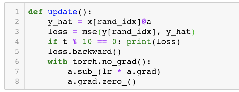
Once you add those, grab a random few points each time, those random few points are called your mini-batch, and that approach is called SGD for Stochastic Gradient Descent.
Vocabulary [1:49:40]
There's quite a bit of vocab we've just covered, so let's remind ourselves.
Learning rate: A thing we multiply our gradient by to decide how much to update the weights by.
Epoch: One complete run through all of our data points (e.g. all of our images). So for non-stochastic gradient descent we just did, every single loop, we did the entire dataset. But if you've got a dataset with a thousand images and our mini-batch size is 100, then it would take you 10 iterations to see every image once. So that would be one epoch. Epochs are important because if you do lots of epochs, then you are looking at your images lots of times, so every time you see an image, there's a bigger chance of overfitting. So we generally don't want to do too many epochs.
Mini-batch: A random bunch of points that you use to update your weights.
SGD: Gradient descent using mini-batches.
Model / Architecture: They kind of mean the same thing. In this case, our architecture is
﹣ the architecture is the mathematical function that you're fitting the parameters to. And we're going to learn later today or next week what the mathematical function of things like ResNet-34 actually is. But it's basically pretty much what you've just seen. It's a bunch of matrix products.
Parameters / Coefficients / Weights: Numbers that you are updating.
Loss function: The thing that's telling you how far away or how close you are to the correct answer. For classification problems, we use cross entropy loss, also known as negative log likelihood loss. This penalizes incorrect confident predictions, and correct unconfident predictions.
These models / predictors / teddy bear classifiers are functions that take pixel values and return probabilities. They start with some functional form like and they fit the parameter
a using SGD to try and do the best to calculate your predictions. So far, we've learned how to do regression which is a single number. Next we'll learn how to do the same thing for classification where we have multiple numbers, but basically the same.
In the process, we had to do some math. We had to do some linear algebra and calculus and a lot of people get a bit scared at that point and tell us "I am not a math person". If that's you, that's totally okay. But you are wrong. You are a math person. In fact, it turns out that in the actual academic research around this, there are not "math people" and "non-math people". It turns out to be entirely a result of culture and expectations. So you should check out Rachel's talk:
There is no such thing as "not a math person"
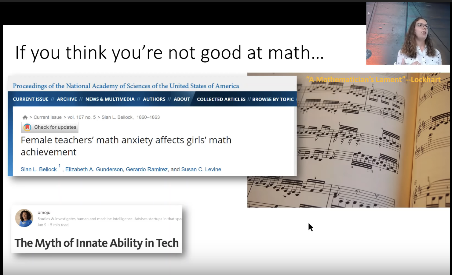
She will introduce you to some of that academic research. If you think of yourself as not a math person, you should watch this so that you learn that you're wrong that your thoughts are actually there because somebody has told you you're not a math person. But there's actually no academic research to suggest that there is such a thing. In fact, there are some cultures like Romania and China where the "not a math person" concept never even appeared. It's almost unheard of in some cultures for somebody to say I'm not a math person because that just never entered that cultural identity.
So don't freak out if words like derivative, gradient, and matrix product are things that you're kind of scared of. It's something you can learn. Something you'll be okay with.
Underfitting and Overfitting [1:54:42]
The last thing I want to close with is the idea of underfitting and overfitting. We just fit a line to our data. But imagine that our data wasn't actually line shaped. So if we try to fit which was something like constant + constant times X (i.e. a line) to it, it's never going to fit very well. No matter how much we change these two coefficients, it's never going to get really close.
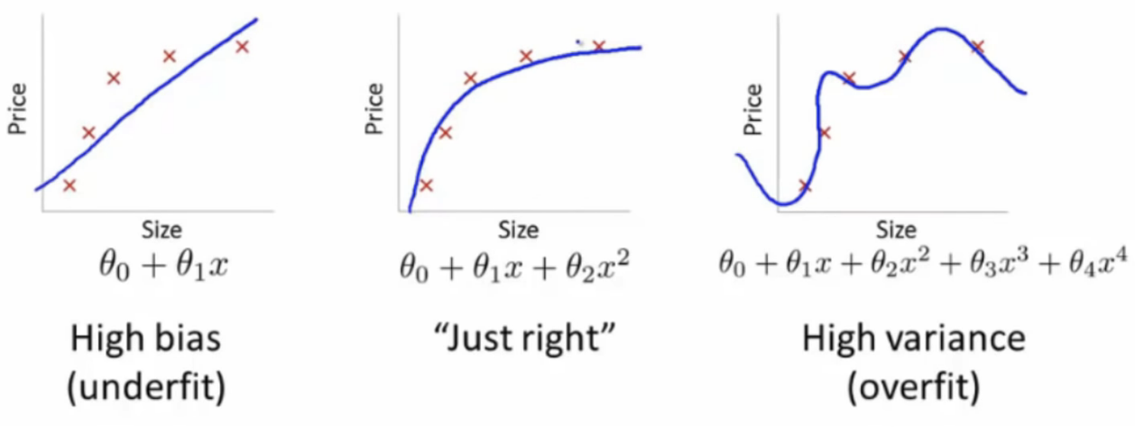
On the other hand, we could fit some much bigger equation, so in this case it's a higher degree polynomial with lots of wiggly bits. But if we did that, it's very unlikely we go and look at some other place to find out the temperature and how much ice cream they are selling and we will get a good result. Because the wiggles are far too wiggly. So this is called overfitting.
We are looking for some mathematical function that fits just right to stay with a teddy bear analogies. You might think if you have a statistics background, the way to make things it just right is to have exactly the same number of parameters (i.e. to use a mathematical function that doesn't have too many parameters in it). It turns out that's actually completely not the right way to think about it.
Regularization and Validation Set [1:56:07]
There are other ways to make sure that we don't overfit. In general, this is called regularization. Regularization or all the techniques to make sure when we train our model that it's going to work not only well on the data it's seen but on the data it hasn't seen yet. The most important thing to know when you've trained a model is actually how well does it work on data that it hasn't been trained with. As we're going to learn a lot about next week, that's why we have this thing called a validation set.
What happens with the validation set is that we do our mini-batch SGD training loop with one set of data with one set of teddy bears, grizzlies, black bears. Then when we're done, we check the loss function and the accuracy to see how good is it on a bunch of images which were not included in the training. So if we do that, then if we have something which is too wiggly, it will tell us. "Oh, your loss function and your error is really bad because on the bears that it hasn't been trained with, the wiggly bits are in the wrong spot." Or else if it was underfitting, it would also tell us that your validation set is really bad.
Even for people that don't go through this course and don't learn about the details of deep learning, if you've got managers or colleagues at work who are wanting to learn about AI, the only thing that you really need to be teaching them is about the idea of a validation set. Because that's the thing they can then use to figure out if somebody's telling them snake oil or not. They hold back some data and they get told "oh, here's a model that we're going to roll out" and then you say "okay, fine. I'm just going to check it on this held out data to see whether it generalizes." There's a lot of details to get right when you design your validation set. We will talk about them briefly next week, but a more full version would be in Rachel's piece on the fast.ai blog called How (and why) to create a good validation set. And this is also one of the things we go into in a lot of detail in the intro to machine learning course. So we're going to try and give you enough to get by for this course, but it is certainly something that's worth deeper study as well.
Thanks everybody! I hope you have a great time building your web applications. See you next week.