Lesson 1 - Image Recognition
These are my personal notes from fast.ai Live (the new International Fellowship programme) course and will continue to be updated and improved if I find anything useful and relevant while I continue to review the course to study much more in-depth. Thanks for reading and happy learning!
Live date: 23 Oct 2018, GMT+8
Topics
- Introduction and welcome!
- fast.ai course v3 website
- Getting started
- Using a GPU
- Jupyter notebook
- Our forums
- PyTorch and fastai library
- Server setup
- fastai v1 documentations
- Advice
- Look at the data
- Training
- Transfer learning
- Interpreting the results
- ResNet50
- Homework
Lesson Resources
- Course website
- Lesson 1 video player
- Video
- Official resources and updates (Wiki)
- Forum discussion
- FAQ, resources, and official course updates
- Jupyter Notebook and code
- Documentations for the fastai deep learning library
Assignments
- Get your GPU going
- Run lesson 1 notebook,
lesson1-pets.ipynb. - Build your own image dataset.
- Try out the different ways of creating datasets.
- Write a guide on how to do it.
- Replicate lesson 1 notebook:
- Reuse the code.
- Repeat process on your own dataset or with a different dataset
- Share your work on forums
- Get on the forum and tell us any little success you had.
- fastai v1 docs
- git clone fastai_docs repo
- run the code
- experiment
Other Resources
Papers
- Optional reading
Blog Posts and Articles
- Optional reading
- fast.ai software could radically democratize AI
- Cricket vs. Baseball - an example by Nikhil Balaji of what you are going to be able to do by the end of lesson 1
- AI Can Recognize Images. But Can It Understand This Headline?
- Towards Natural Language Semantic Code Search by Hamel Husain and team at GitHub Engineering
- fast.ai recent alumni, Christine Payne, now at OpenAI and her project, Clara, a neural network generator
- One of our other alumni (Sanyam Bhutani) of the course recently interviewed with OpenAI Fellow: Christine McLeavey Payne
- A small team of student AI coders beats Google’s machine-learning code
My Notes
Getting Started
Welcome! Practical Deep Learning for Coders lesson 1.
[0:12] There's a lesson 0. Lesson 0 is why do you need GPU and how did you get it setup. So if you haven't got a GPU running yet, then go back and do that.
💡 Note: you can also watch this first lesson without following along with a GPU, so you can see how it all works. Then watch a 2nd time after you have a GPU and try to implement the code yourself.
Make sure your GPU environment is set up and you can run Jupyter Notebook. Then you are ready to start the real lesson 1.
The code is in Python.
Four shortcuts:
- Shift+Enter: runs the code or markdown on a cell
- Up Arrow+Down Arrow: toggle across cells
- b: create new cell
- 0+0: restart kernel
[2:45]
Jupyter Notebook is a really interesting device for data scientists because it lets you run interactive experiments and give you not just a static piece of information but something you can interactively experiment with.
How to use notebooks and the materials well based on the last three years of experience:
- Just watch a lesson end to end.
- Don't try to follow along because it's not really designed to go the speed where you can follow along. It's designed to be something where you just take in the information, you get a general sense of all the pieces, how it all fits together.
- Then you can go back and go through it more slowly pausing the video, trying things out, making sure that you can do the things that I'm doing and you can try and extend them to do things in your own way.
- Don't worry if things are zipping along faster than you can do them. That's normal.
- Don't try and stop and understand everything the first time. If you do understand everything the first time, good for you. But most people don't particularly as the lessons go on, they get faster and they get more difficult.
So at this point, we've got our notebooks going. We're ready to start doing deep learning.
You can do deep learning [4:31]
The main thing that hopefully you're going to agree at the end of this is that you can do world-class practitioner level deep learning regardless of who you are.
Main places to be looking for things are:
- course-v3.fast.ai
- you can find out how to get a GPU and other information.
- forums
Who is Jeremy Howard? [5:27]
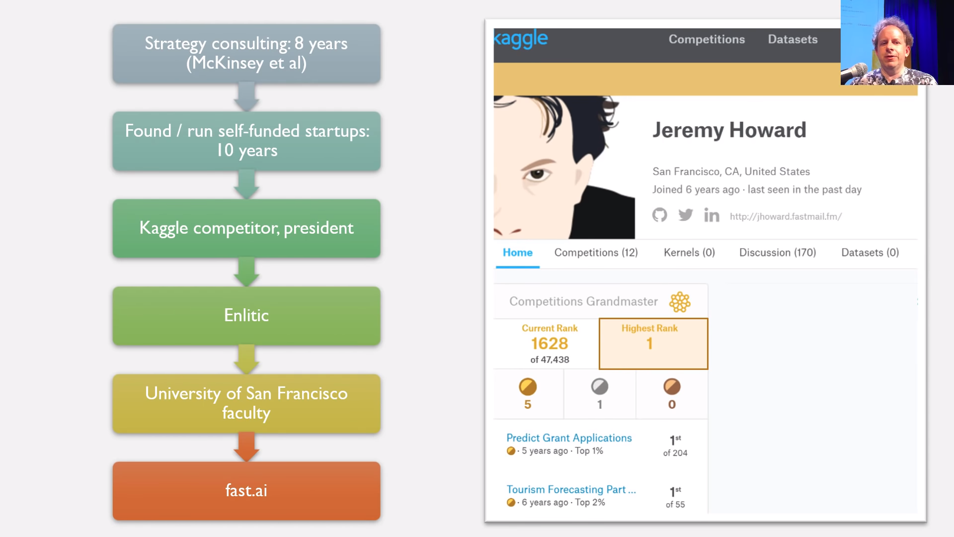
A little bit about why we should listen to Jeremy.
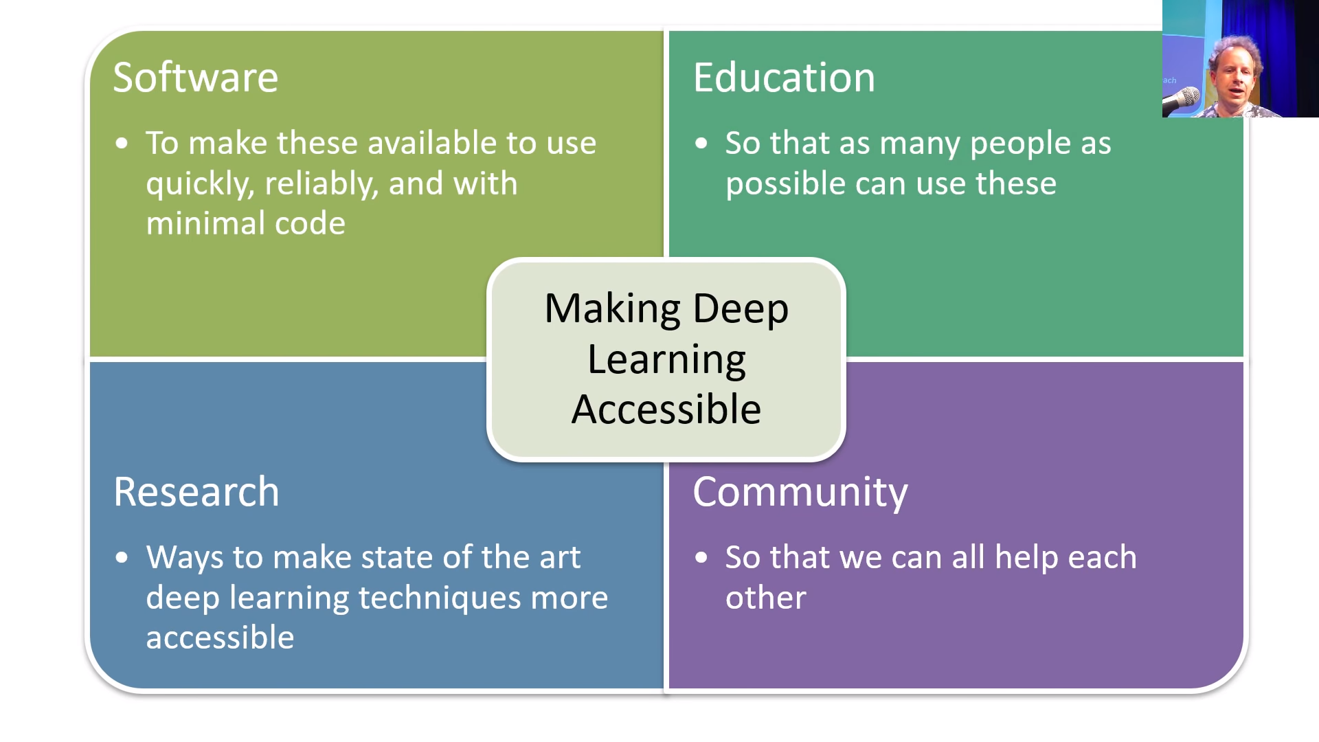
Using machine learning to do useful things [6:48]
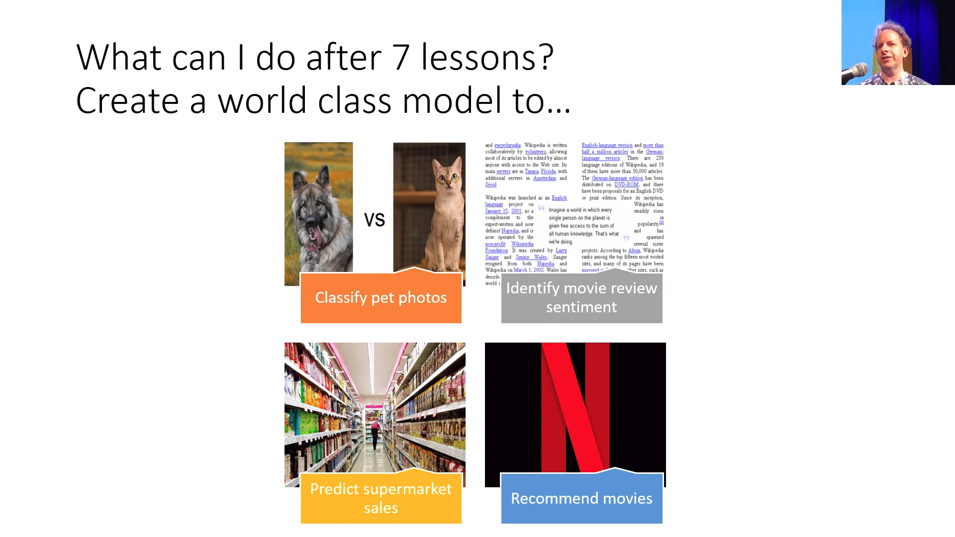
What can I do after 7 lessons? [7:25]
There is a lot as to how much people put into this. Jeremy knows a lot of people who work full-time on fast AI. Some folks whose do the two parts can spend a whole year doing it really intensively. Jeremy knows some folks watch the videos on double-speed and never do any homework and come at the end of it with a general sense of what's going on. So, there's lots of different ways you can do this.
If you follow along with 10 hours a week or so approach for the 7 weeks, by the end, you will be able to:
- Build an image classification model on pictures that you choose that will work at a world class level.
- Classify text using whatever datasets you're interested in.
- Make predictions of commercial applications like sales.
- Build recommendation systems such as the one used by Netflix.
Not toy examples of any of these but actually things that can come top 10 in Kaggle competitions, that can beat everything that's in the academic community.
The prerequisite is one year of coding and high school math.
Myths about Deep Learning and AI [9:05]
This lesson breaks down the previously held myths about Deep Learning and AI which are no longer true—now, literally anyone with a computer can learn.
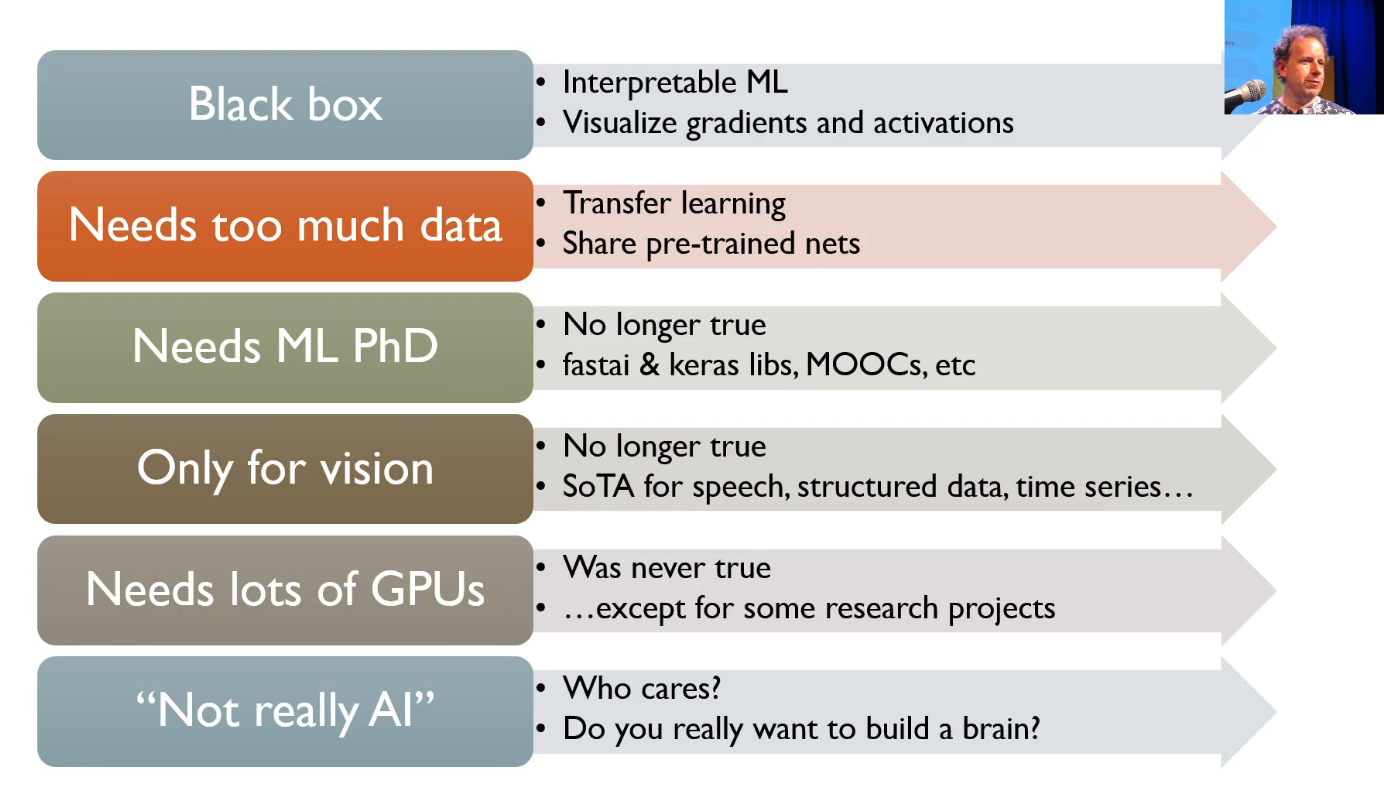
You will probably hear a lot of naysayers, less now than a couple of years ago than we started. A lot of them telling you that you can't do it or you shouldn't be doing it or that deep learning got all these problems. It's not perfect. These are all things that people claim about, which are either pointless or untrue.
- It's not a black box. It's really great for interpreting what's going on.
- It does not need much data for most practical applications.
- You don't need a PhD. Rachel has one so it doesn't actually stop you from doing deep learning if you have a PhD.
- It can be used very widely for lots of different applications, not just for vision.
- You don't need lots of hardware. 36 cents an hour server is more than enough to get world-class results for most problems.
- It is true that maybe this is not going to help you build a sentient brain, but that's not our focus. For all the people who say deep learning is not interesting because it's not really AI, not really a conversation that Jeremy interested in. We are focused on solving interesting real-world problems.
What are you going to be able to do by the end of lesson 1 [10:24]
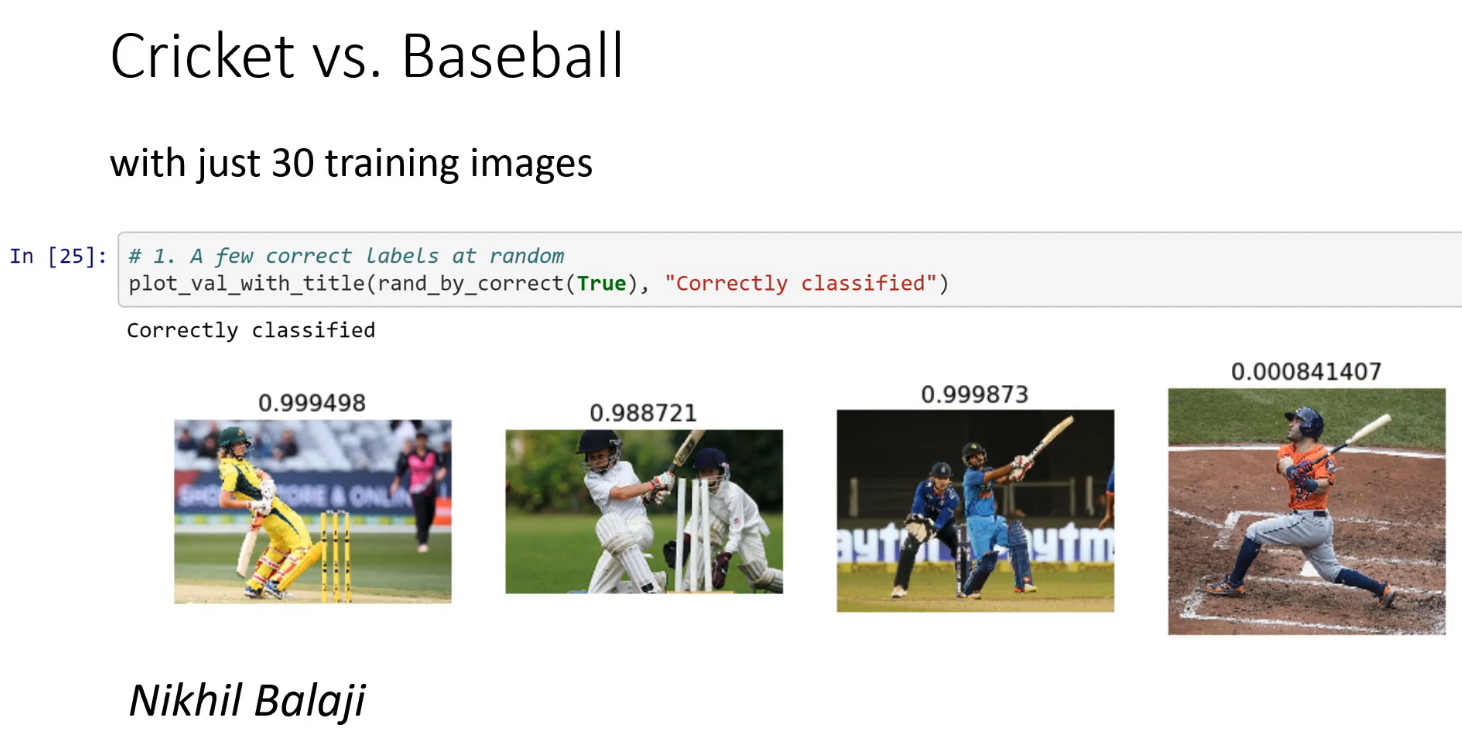
Cricket vs Baseball - an example by Nikhil of what you are going to be able to do by the end of lesson 1.
Topdown approach [11:02]
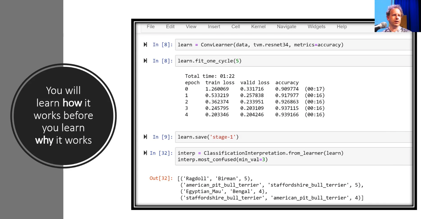
You will learn how it works before you learn why it works.
We are going to start by looking at code which is different to many of academic courses. We are going to learn to build a useful thing today. That means that at the end of today, you won't know all the theory. There will be lots of aspects of what we do that you don't know why or how it works. That's okay! You will learn why and how it works over the next 7 weeks. But for now, we've found that what works really well is to actually get your hands dirty coding—not focusing on theory. Because, it's still a situation where people who are good practitioners have a really good feel for how to work with code and how to work with data and you can only get that through experience. The best way to get that feel of how to get good models is to create lots of models through lots of coding and study them carefully. So, let's try that, let's try getting started.
What's your pet [12:26]
Open your Jupyter Notebook and click on lesson1-pets.ipynb.
Real deep learning practitioners know the keyboard shortcuts. The keyboard shortcut is:
Shift+Enter to run a cell.We are going to go through this quickly and later on we're going to go back over it more carefully. Here's the quick version to get a sense of what's going on. So, here we are in lesson 1.
These three lines is what we start every notebook with:
%reload_ext autoreload
%autoreload 2
%matplotlib inline
These things starting % are special directives to Jupyter Notebook itself, they are not Python code. They are called "magics". The details aren't very important but basically it says:
- If somebody changes underlying library code while I'm running this, please reload it automatically.
- If somebody asks to plot something, then please plot it here in this Jupyter Notebook.
[14:00] The next two lines load up the fastai library:
from fastai import *
from fastai.vision import *
What is fastai library? If you go to docs.fast.ai, this is the fastai library:
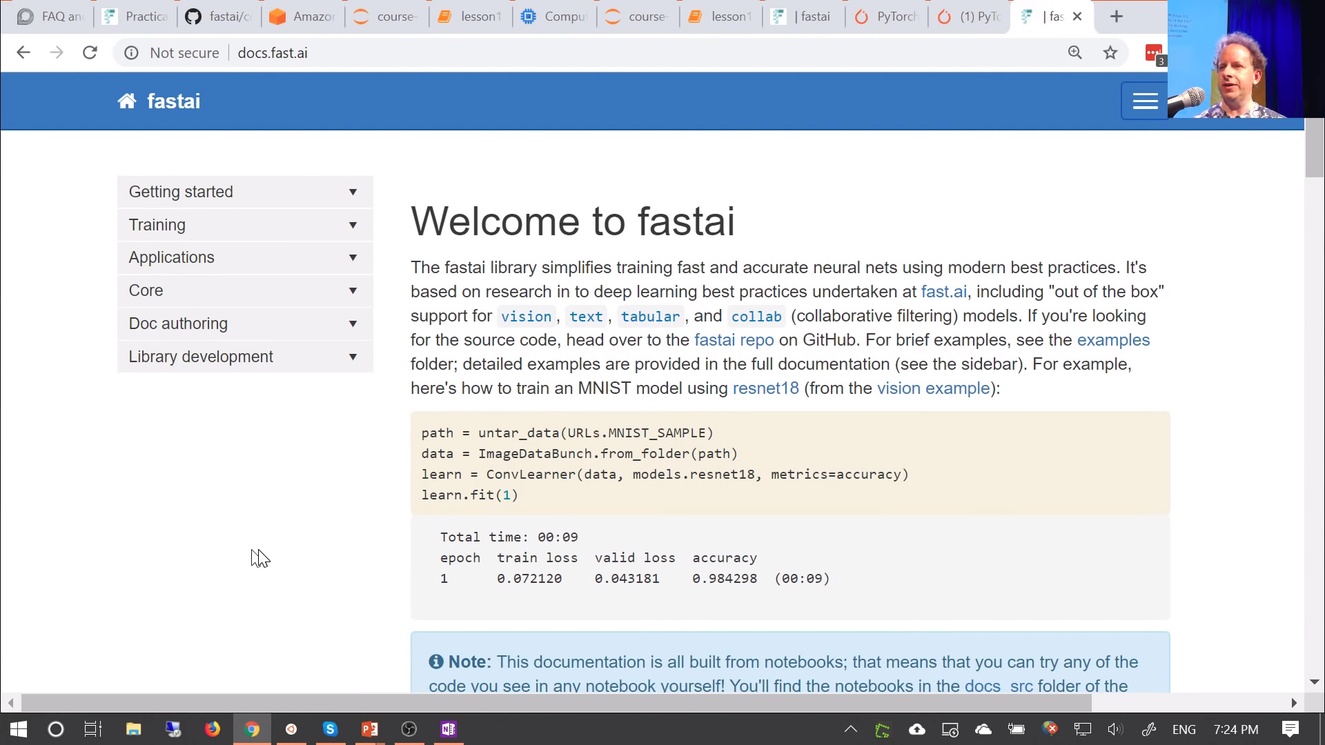
Everything we are going to do is going to be using either fastai or PyTorch which fastai sits on top of. PyTorch is fast growing extremely popular library. It's a bit newer than TensorFlow, so in a lot of ways it's more modern than TensorFlow. We use it because we used to use TensorFlow a couple years ago and we found we can do a lot more, a lot more quickly with PyTorch.
Currently fastai supports four applications:
- Computer vision
- Natural language text
- Tabular data
- Collaborative filtering
[15:45]
import * - If you are a Python software engineer, you probably feeling sick because this is something you've all been told to never ever do.
There are very good reasons to not use import * in standard production code with most libraries. But things like MATLAB is the opposite. Everything is there for you all the time. You don't even have to import things a lot of the time. It's kind of funny - we've got these two extremes of how do I code. The scientific programming community has one way, and then software engineering community has the other. Both have really good reasons for doing things.
With the fastai library, we actually support both approaches. In Jupyter Notebook where you want to be able to quickly interactively try stuff out, you don't want to constantly going back up to the top and importing more stuff. You want to be able to use lots of tab complete and be very experimental, so import * is great. When you are building stuff in production, you can do the normal PEP8 style proper software engineering practices. This is a different style of coding. It's not that there are no rules in data science programming, the rules are different. When you're training models, the most important thing is to be able to interactively experiment quickly. So you will see we use a lot of different processes, styles, and stuff to what you are used to. But they are there for a reason and you'll learn about them over time.
The other thing to mention is that the fastai library is designed in a very interesting modular way and when you do use import *, there's far less clobbering of things than you might expect. It's all explicitly designed to allow you to pull in things and use them quickly without having problems.
Looking at the data [17:56]
Two main places that we will be tending to get data from for the course:
- Academic datasets
- Academic datasets are really important. They are really interesting. They are things where academics spend a lot of time curating and gathering a dataset so that they can show how well different kinds of approaches work with that data. The idea is they try to design datasets that are challenging in some way and require some kind of breakthrough to do them well.
- We are going to start with an academic dataset called the pet dataset.
- Kaggle competition datasets
Both types of datasets are interesting for us particularly because they provide strong baseline. That is to say you want to know if you are doing a good job. So with Kaggle datasets that come from a competition, you can actually submit your results to Kaggle and see how well you would have gone in that competition. If you can get in about the top 10%, then I'd say you are doing pretty well.
Academic datasets, academics write down in papers what the state of the art is so how well did they go with using models on that dataset. So this is what we are going to do. We are going to try to create models that get right up towards the top of Kaggle competitions, preferably in the top 10, not just top 10% or that meet or exceed academic state-of-the-art published results. So when you use an academic dataset, it's important to cite it. Here there's a link to the Oxford-IIIT Pet Dataset paper that it's from. You don't need to read that paper right now, but if you are interested in learning more about it and why it was created and how it was created, all the details are there.
In this case, this is a pretty difficult challenge. The Pet dataset is going to ask us to distinguish between 37 different categories of dog breed and cat breed. So that's really hard. In fact, every course until this one, we've used a different dataset which is one where you just have to decide if something is a dog or a cat. So you've got a 50-50 chance right away and dogs and cats look really different. Or else lots of dog breeds and cat breeds look pretty much the same.
So why have we changed the dataset? We've got to the point now where deep learning is so fast and so easy that the dogs versus cats problem which a few years ago was considered extremely difficult around 80% accuracy was the state of the art, it's now too easy. Our models were basically getting everything right all the time without any tuning and so there weren't really a lot of opportunities for me to show you how to do more sophisticated stuff. So we've picked a harder problem this year.
[20:51]
This kind of thing where you have to distinguish between similar categories is called fine grained classification in the academic context.
untar_data
The first thing we have to do is download and extract the data that we want. We're going to be using this function called untar_data which will download it automatically and untar it. AWS has been kind enough to give us lots of space and bandwidth for these datasets so they'll download super quickly for you.
path = untar_data(URLs.PETS); path
help
The first question then would be how do I know what untar_data does. You could just type help and you will find out what module it came from (since we did import * you don't necessarily know that), what it does, and something you might not have seen before even if you are an experienced programmer is what exactly you pass to it. You're probably used to seeing the names: url, fname, dest, but you might not be used to seeing Union[pathlib.Path, str]. These bits are types and if you're used to typed programming language, you would be used to seeing them, but Python programmers are less used to it. But if you think about it, you don't actually know how to use a function unless you know what type each thing is that you're providing it. So we make sure that we give you that type information directly here in the help.
In this case, url is a string, fname is either path or a string and defaults to nothing (Union means "either"). dest is either a string or a path and defaults to nothing.
help(untar_data)

# -----------------------------------------------------------------------------
# Output
# -----------------------------------------------------------------------------
Help on function untar_data in module fastai.datasets:

untar_data(url:str, fname:Union[pathlib.Path, str]=None, dest:Union[pathlib.Path, str]=None)
    Download `url` if doesn't exist to `fname` and un-tgz to folder `dest`
We'll learn more shortly about how to get more documentation about the details of this, but for now, we can see we don't have to pass in a file name fname or a destination dest, it'll figure them out for us from the URL.
For all the datasets we'll be using in the course, we already have constants defined for all of them (i.e: URLs.PETS). So in this URLs class, you can see where it's going to grab it from.
untar_data will download that to some convenient path and untar it for us and it will then return the value of path.
path = untar_data(URLs.PETS); path

# -----------------------------------------------------------------------------
# Output
# -----------------------------------------------------------------------------
PosixPath('/data1/jhoward/git/course-v3/nbs/dl1/data/oxford-iiit-pet')
In Jupyter Notebook, you can just write a variable on its own (semicolon is just an end of statement in Python) and it prints it. You can also say print(path) but again, we are trying to do everything fast and interactively, so just write it and here is the path where it's given us our data.
Next time you run this, since you've already downloaded it, it won't download it again. Since you've already untared it, it won't untar it again. So everything is designed to be pretty automatic and easy.
[23:50]
There are some things in Python that are less convenient for interactive use than they should be. For example, when you do have a path object, seeing what's in it actually takes a lot more typing than I would like. So sometimes we add functionality into existing Python stuff. One of the things we do is add a ls() method to path.
path.ls()

# -----------------------------------------------------------------------------
# Output
# -----------------------------------------------------------------------------
['annotations', 'images']
These are what's inside this path, so that's what we just downloaded.
Python 3 pathlib [24:25]
path_anno = path/'annotations'
path_img = path/'images'
If you are an experienced Python programmer, you may not be familiar with this approach of using a slash like this. This is a really convenient function that's part of Python 3. It's functionality from pathlib. Path object is much better to use than strings. They let you use basically create sub paths like this. It doesn't matter if you're on Windows, Linux, or Mac. It is always going to work exactly the same way. path_img is the path to the images in that dataset.
[24:57]
So if you are starting with a brand new dataset trying to do some deep learning on it. What do you do? Well, the first thing you would want to do is probably see what's in there. So we found that annotations and images are the directories in there, so what's in this images?
get_image_files [25:15]
There's a lot of functions in fastai for you. There's one called get_image_files that will just grab an array of all of the image files based on extension in a path.
fnames = get_image_files(path_img)
fnames[:5]

# -----------------------------------------------------------------------------
# Output
# -----------------------------------------------------------------------------
[PosixPath('/data1/jhoward/git/course-v3/nbs/dl1/data/oxford-iiit-pet/images/american_bulldog_146.jpg'),
 PosixPath('/data1/jhoward/git/course-v3/nbs/dl1/data/oxford-iiit-pet/images/german_shorthaired_137.jpg'),
 PosixPath('/data1/jhoward/git/course-v3/nbs/dl1/data/oxford-iiit-pet/images/japanese_chin_139.jpg'),
 PosixPath('/data1/jhoward/git/course-v3/nbs/dl1/data/oxford-iiit-pet/images/great_pyrenees_121.jpg'),
 PosixPath('/data1/jhoward/git/course-v3/nbs/dl1/data/oxford-iiit-pet/images/Bombay_151.jpg')]
This is a pretty common way for computer vision datasets to get passed around - just one folder with a whole bunch of files in it. So the interesting bit then is how do we get the labels. In machine learning, the labels refer to the thing we are trying to predict. If we just eyeball this, we could immediately see that the labels are actually part of the file names. It's kind of like path/label_number.extension. We need to somehow get a list of label bits of each file name, and that will give us our labels. Because that's all you need to build a deep learning model:
- Pictures (files containing the images)
- Labels
In fastai, this is made really easy. There is an object called ImageDataBunch. An ImageDataBunch represents all of the data you need to build a model and there's some factory methods which try to make it really easy for you to create that DataBunch - a training set, a validation set with images and labels.
In this case, we need to extract the labels from the names. We are going to use from_name_re. re is the module in Python that does regular expressions - things that's really useful for extracting text.
Here is the regular expression that extract the label for this dataset:
np.random.seed(2)
pat = r'/([^/]+)_\d+.jpg$'
Regular expressions or in short regex is a way to search a string in text using pattern matching methods.
Let's deconstruct this regex pattern, /([^/]+)_\d+.jpg$ by reading it backwards:
| Expression | Explaination |
|---|---|
$ | end of search |
.jpg | last chars to be found in search string, also right file format checking |
\d | numerical digits, + sign denotes can be one or more of them |
_ | should come before start of digits |
() | denotes group of characters |
[] | denotes another subgroup if characters in previous group |
^/ | ^ denotes negation , so + says all other chars except / |
( [ ^/ ] + ) | searches all characters except / |
/ | first / in regex says, end of search |
Considering search string was PosixPath('images/japanese_chin_139.jpg'), this regex pattern will give us string japanese_chin.
With this factory method, we can basically say:
path_img: a path containing imagesfnames: a list of file namespat: a regular expression (i.e. pattern) to be used to extract the label from the file nameds_tfms: we'll talk about transforms latersize: what size images do you want to work with.
That might seem weird because images have size. This is a shortcoming of current deep learning technology which is that a GPU has to apply the exact same instruction to a whole bunch of things at the same time in order to be fast. If the images are different shapes and sizes, you can't do that. So we actually have to make all of the images the same shape and size. In part 1 of the course, we are always going to be making images square shapes. Part 2, we will learn how to use rectangles as well. It turns out to be surprisingly nuanced. But pretty much everybody in pretty much all computer vision modeling nearly all of it uses this approach of square. 224 by 224, for reasons we'll learn about, is an extremely common size that most models tend to use so if you just use size=224, you're probably going to get pretty good results most of the time. This is kind of the little bits of artisanship that I want to teach you which is what generally just works. So if you just use size 224, that'll generally just work for most things most of the time.
data = ImageDataBunch.from_name_re(path_img, fnames, pat, ds_tfms=get_transforms(), size=224)
data.normalize(imagenet_stats)
[29:16]
ImageDataBunch.from_name_re is going to return a DataBunch object. In fastai, everything you model with is going to be a DataBunch object. Basically DataBunch object contains 2 or 3 datasets - it contains your training data, validation data, and optionally test data. For each of those, it contains your images and your labels, your texts and your labels, or your tabular data and your labels, or so forth. And that all sits there in this one place (i.e. data).
Something we will learn more about in a little bit is normalization. But generally in nearly all machine learning tasks, you have to make all of your data about the same "size" - they are specifically about the same mean and standard deviation. So there is a normalize function that we can use to normalize our DataBunch in that way.
[30:25]
Question❓: What does the function do if the image size is not 224?
This is what we are going to learn about shortly. Basically this thing called transforms (i.e. ds_tfms=get_transforms()) is used to do a number of the things and one of the things it does is to make something size 224.
data.show_batch
Let's take a look at a few pictures. Here are a few pictures of things from my DataBunch. So you can see data.show_batch can be used to show me some of the contents in my DataBunch. So you can see roughly what's happened is that they all seem to have being zoomed and cropped in a reasonably nice way. So basically what it'll do is something called by default center cropping which means it'll grab the middle bit and it'll also resize it. We'll talk more about the detail of this because it turns out to actually be quite important, but basically a combination of cropping and resizing is used.
data.show_batch(rows=3, figsize=(7,6))
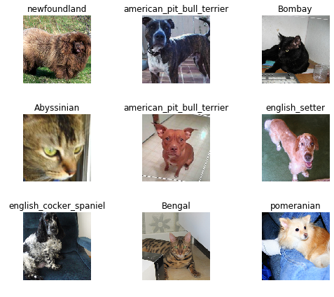
Something else we are going to learn about is we also use this to do something called data augmentation. So there's actually some randomization in how much and where it crops and stuff like that.
Basic the basic idea is some cropping, resizing, and padding. So there's all kinds of different ways it depends on data augmentation which we are going to learn about shortly.
[31:51] Question❓: What does it mean to normalize the images?
Normalizing the images, we're going to be learning more about later in the course, but in short, it means that the pixel values start out from naught (0) to 255. And some channels might tend to be really bright, some might tend to be really not bright at all, some might vary a lot, and some might not very much at all. It really helps train a deep learning model if each one of those red green and blue channels has a mean of zero and a standard deviation of one.
If your data is not normalized, it can be quite difficult for your model to train well. So if you have trouble training a model, one thing to check is that you've normalized it.
[33:00] Question❓: As GPU mem will be in power of 2, doesn't size 256 sound more practical considering GPU utilization compared to 224?
The brief answer is that the models are designed so that the final layer is of size 7 by 7, so we actually want something where if you go 7 times 2 a bunch of times (224 = 72222*2), then you end up with something that's a good size.
[33:27]
We will get to all these details but the key thing is I wanted to get to training a model as quickly as possible.
It is important to look at the data
One of the most important thing to be a really good practitioner is to be able to look at your data. So it's really important to remember to go data.show_batch and take a look. It's surprising how often when you actually look at the dataset you've been given that you realize it's got weird black borders on it, some of the things have text covering up some of it, or some of it is rotated in odd ways. So make sure you take a look.
The other thing we want to do at is to look at the labels. All of the possible label names are called your classes. With DataBunch, you can print out your data.classes.
print(data.classes)
len(data.classes),data.c

# -----------------------------------------------------------------------------
# Output
# -----------------------------------------------------------------------------
['american_bulldog', 'german_shorthaired', 'japanese_chin', 'great_pyrenees', 'Bombay', 'Bengal', 'keeshond', 'shiba_inu', 'Sphynx', 'boxer', 'english_cocker_spaniel', 'american_pit_bull_terrier', 'Birman', 'basset_hound', 'British_Shorthair', 'leonberger', 'Abyssinian', 'wheaten_terrier', 'scottish_terrier', 'Maine_Coon', 'saint_bernard', 'newfoundland', 'yorkshire_terrier', 'Persian', 'havanese', 'pug', 'miniature_pinscher', 'Russian_Blue', 'staffordshire_bull_terrier', 'beagle', 'Siamese', 'samoyed', 'chihuahua', 'Egyptian_Mau', 'Ragdoll', 'pomeranian', 'english_setter']

(37, 37)
That's all of the possible labels that we found by using that regular expression on the file names. We learnt earlier on at the top that there are 37 possible categories, so just checking len(data.classes), it is indeed 37. DataBunch will always have a property called c. We will get to the technical detail later, but for now, you can kind of think of it as being the number of classes. For things like regression problems and multi-label classification, that's not exactly accurate, but it'll do for now. It is important to know that data.c is a really important piece of information that is something like, or at least for classification problems it is, the number of classes.
Training [35:07]
Believe it or not, we are now ready to train a model. A model is trained in fastai using something called a "learner".
- DataBunch: A general fastai concept for your data, and from there, there are subclasses for particular applications like
ImageDataBunch. - Learner: A general concept for things that can learn to fit a model. From that, there are various subclasses to make things easier in particular, there is a
ConvLearnerwhich is something that will create a convolutional neural network for you.
📢 2018-10-29: there's been one change to fastai v1.0.15 and above—ConvLearner is now called create_cnn. You'll need to make that change in any notebooks that you've created too. Reference: forum: lesson 1 official resources and updates
learn = create_cnn(data, models.resnet34, metrics=error_rate)
For now, just know that to create a learner for a convolutional neural network, you just have to tell it two things:
data: What's your data. Not surprisingly, it takes a DataBunch.arch: What's your architecture. There are lots of different ways of constructing a convolutional neural network.
For now, the most important thing for you to know is that there's a particular kind of model called ResNet which works extremely well nearly all the time. For a while, at least, you really only need to be doing choosing between two things which is what size ResNet do you want. There are ResNet34 and ResNet50. When we are getting started with something, I'll pick a smaller one because it'll train faster. That's as much as you need to know to be a pretty good practitioner about architecture for now which is that there are two variants of one architecture that work pretty well: ResNet34 and ResNet50. Start with a smaller one and see if it's good enough.
That is all the information we need to create a convolutional neural network learner.
There is one other thing I'm going to give it though which is a list of metrics. Metrics are literally just things that gets printed out as it's training. So I'm saying I would like you to print out error rate.
[37:25]
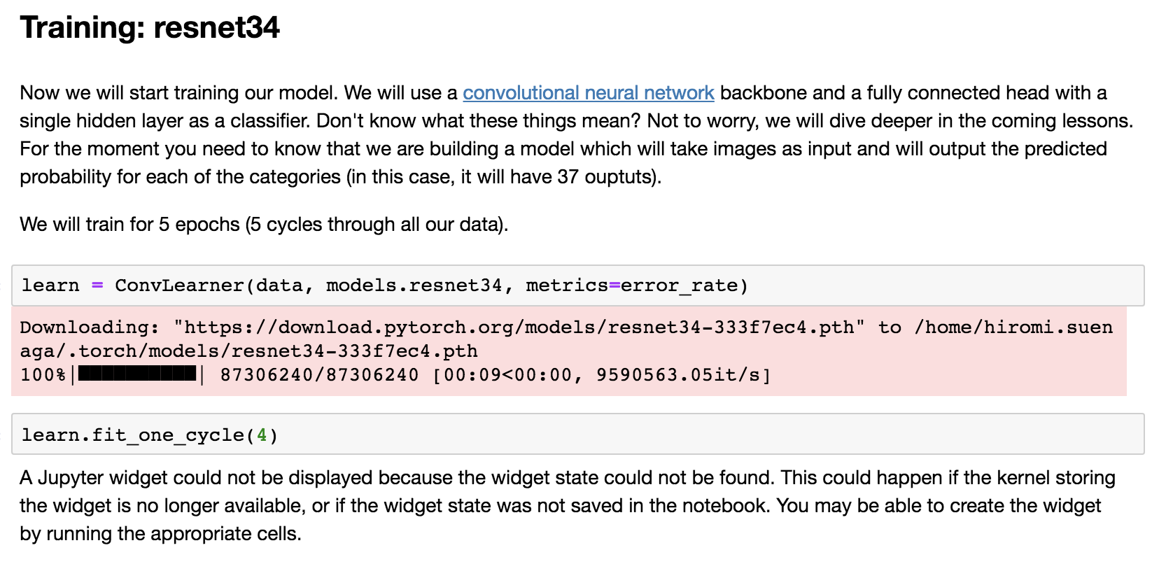
The first time I run this on a newly installed box, it downloads the ResNet34 pre-trained weights. What that means is that this particular model has actually already been trained for a particular task. And that particular task is that it was trained on looking at about one and a half million pictures of all kinds of different things, a thousand categories of things, using an image dataset called ImageNet. So we can download those pre-trained weights so that we don't start with a model that knows nothing about anything, but we actually start with a model that knows how to recognize a thousand categories of things in ImageNet. I don't think all of these 37 categories of pet are in ImageNet but there were certainly some kinds of dog and some kinds of cat. So this pre-trained model knows quite a little bit about what pets look like, and it certainly knows quite a lot about what animals look like and what photos look like. So the idea is that we don't start with a model that knows nothing at all, but we start by downloading a model that knows something about recognizing images already. So it downloads for us automatically, the first time we use it, a pre-trained model and then from now on, it won't need to download it again - it'll just use the one we've got.
Transfer learning [38:54]
❗❗❗ This is really important. We are going to learn a lot about this. It's kind of the focus of the whole course which is how to do this thing called "transfer learning."
How to take a model that already knows how to do something pretty well and make it so that it can do your thing really well. We will take a pre-trained model, and then we fit it so that instead of predicting a thousand categories of ImageNet with ImageNet data, it predicts the 37 categories of pets using your pet data. By doing this, you can train models in 1/100 or less of the time of regular model training with 1/100 or less of the data of regular model training. Potentially, many thousands of times less. Remember I showed you the slide of Nikhil's lesson 1 project from last year? He used 30 images. There are not cricket and baseball images in ImageNet but it turns out that ImageNet is already so good at recognizing things in the world that just 30 examples of people playing baseball and cricket was enough to build a nearly perfect classifier.
Overfitting [40:05]
Wait a minute, how do you know it can actually recognize pictures of people playing cricket versus baseball in general? Maybe it just learnt to recognize those 30. Maybe it's just cheating. That's called "overfitting". We'll be talking a lot about that during this course. But overfitting is where you don't learn to recognize pictures of say cricket versus baseball, but just these particular cricketers in these particular photos and these particular baseball players in these particular photos. We have to make sure that we don't overfit. The way to do that is using something called a validation set. A validation set is a set of images that your model does not get to look at. So these metrics (e.g. error_rate) get printed out automatically using the validation set - a set of images that our model never got to see. When we created our DataBunch, it automatically created a validation set for us. We'll learn lots of ways of creating and using validation sets, but because we're trying to bake in all of the best practices, we actually make it nearly impossible for you not to use a validation set. Because if you're not using a validation set, you don't know if you're overfitting. So we always print out the metrics on a validation, we've always hold it out, we always make sure that the model doesn't touch it. That's all done for you, and all built into this DataBunch object.
Fitting your model [41:40]
So now we have a ConvLearner, we can fit it. You can just use a method called fit but in practice, you should nearly always use a method called fit_one_cycle. In short, one cycle learning is a paper that was released in Mar 2018 and turned out to be dramatically better both more accurate and faster than any previous approach. Again, I don't want to teach you how to do 2017 deep learning. In 2018, the best way to fit models is to use something called one cycle.
For now, just know that this number, 4, basically decides how many times do we go through the entire dataset, how many times do we show the dataset to the model so that it can learn from it. Each time it sees a picture, it's going to get a little bit better. But it's going to take time and it means it could overfit. If it sees the same picture too many times, it will just learn to recognize that picture, not pets in general. We'll learn all about how to tune this number during the next couple of lessons but starting out with 4 is a pretty good start just to see how it goes and you can actually see after four epochs or four cycles, we got an error rate of 6%. And it took 1 minute and 56 seconds.
learn.fit_one_cycle(4)

# -----------------------------------------------------------------------------
# Output
# -----------------------------------------------------------------------------
Total time: 01:10
epoch  train loss  valid loss  error_rate
1      1.175709    0.318438    0.099800    (00:18)
2      0.492309    0.229078    0.075183    (00:17)
3      0.336315    0.211106    0.067199    (00:17)
4      0.233666    0.191813    0.057219    (00:17)
So 94% of the time, we correctly picked the exact right one of those 94 dog and cat breeds which feels pretty good to me.
[44:29] But to get a sense of how good it is, maybe we should go back and look at the paper.
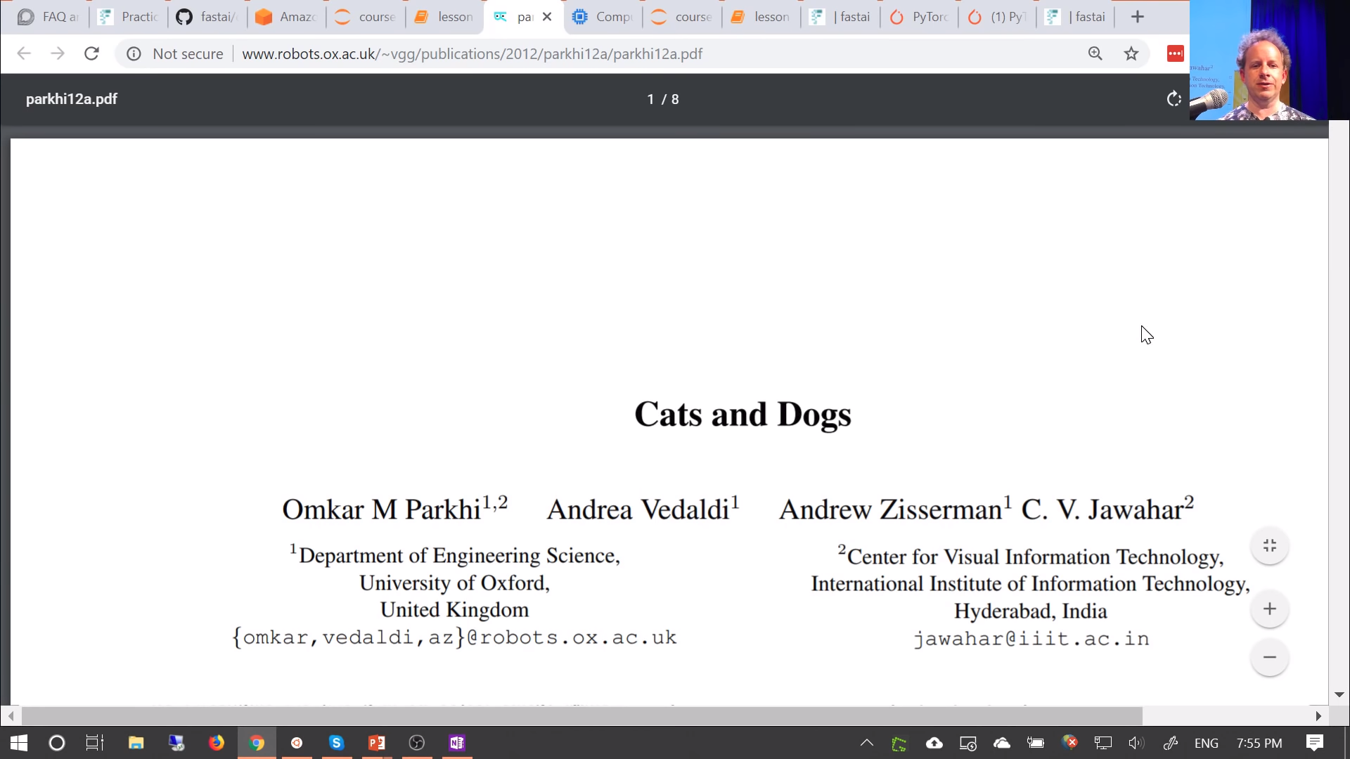
Remember, I said the nice thing about using academic papers or Kaggle dataset is we can compare our solution to whatever the best people in Kaggle did or in the academics did. This particular dataset of pet breeds is from 2012 and if I scroll through the paper, you'll generally find in any academic paper there'll be a section called experiments about 2/3 of the way through. If you find a section on experiments, then you can find a section on accuracy and they've got lots of different models and their models. The models as you'll read about in the paper, it's really pet specific. They learn something about how pet heads look and how pet bodies look, and pet image in general look. And they combine them all together and once they use all of this complex code and math, they got an accuracy of 59%. So in 2012, this highly pet specific analysis got an accuracy of 59%. These were the top researchers from Oxford University. Today in 2018, with basically about three lines of code, we got 94% (i.e. 6% error). So that gives you a sense of how far we've come with deep learning, and particularly with PyTorch and fastai, how easy things are.
[46:43] We just trained a model. We don't know exactly what that involved or how it happened but we do know that with 3 or 4 lines of code, we've built something which smashed the accuracy of the state-of-the-art of 2012. 6% error certainly sounds like pretty impressive for something that can recognize different dog breeds and cat breeds, but we don't really know why it works, but we will. That's okay.
Getting the most out of this course
The number one regret of past students:
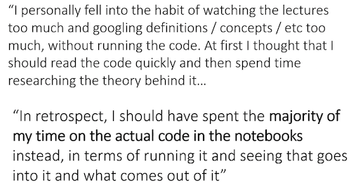
❗❗❗ So please run the code. Really run the code. ❗❗❗ [47:54]
Your most important skills to practice are learning and understanding what goes in and what comes out.
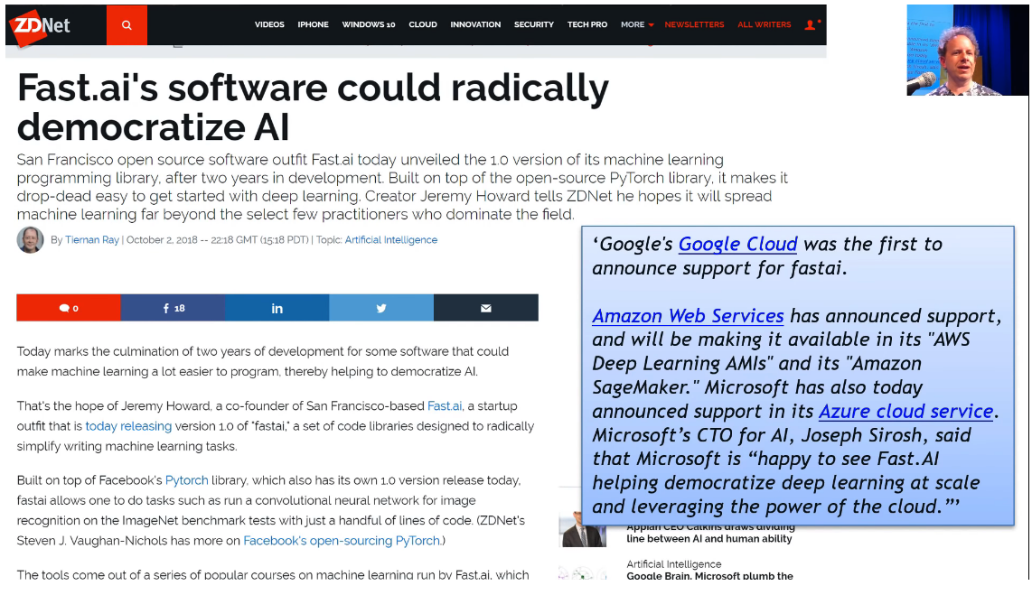
Fastai library is pretty new, but it's getting an extraordinary amount of traction. It's making a lot of things a lot easier, but it's also making new things possible. So really understanding the fastai software is something which is going to take you a long way. And the best way to really understand the fastai software well is by using the fastai documentation.
Keras [49:25]
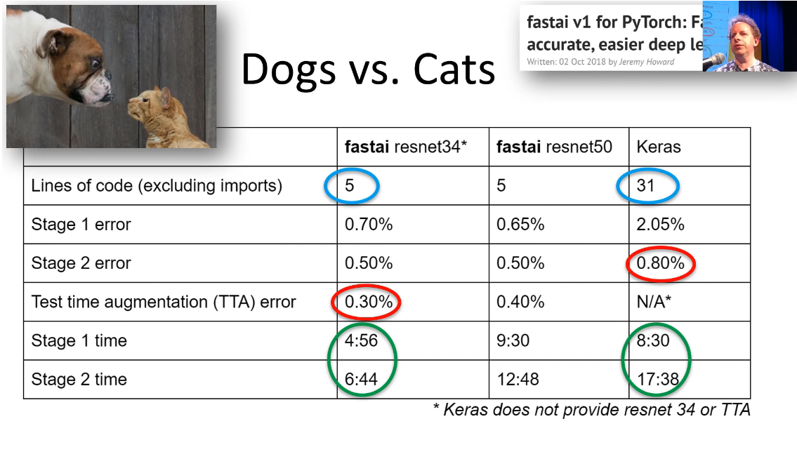
So how does it compare? There's only one major other piece of software like fastai that tries to make deep learning easy to use and that's Keras. Keras is a really terrific piece of software, we actually used it for the previous courses until we switch to fastai. It runs on top of TensorFlow. It was the gold standard for making deep learning easy to use before. But life is much easier with fastai. So if you look at the last year's course exercise which is getting dogs vs. cats, fastai lets you get much more accurate (less than half the error on a validation set), training time is less than half the time, lines of code is about 1/6. The lines of code are more important than you might realize because those 31 lines of Keras code involved you making a lot of decisions, setting lots of parameters, doing lots of configuration. So that's all stuff where you have to know how to set those things to get best practice results. Or else, those 5 lines of code, any time we know what to do for you, we do it for you. Anytime we can pick a good default, we pick it for you. So hopefully you will find this a really useful library, not just for learning deep learning but for taking it a very long way.
[50:53]
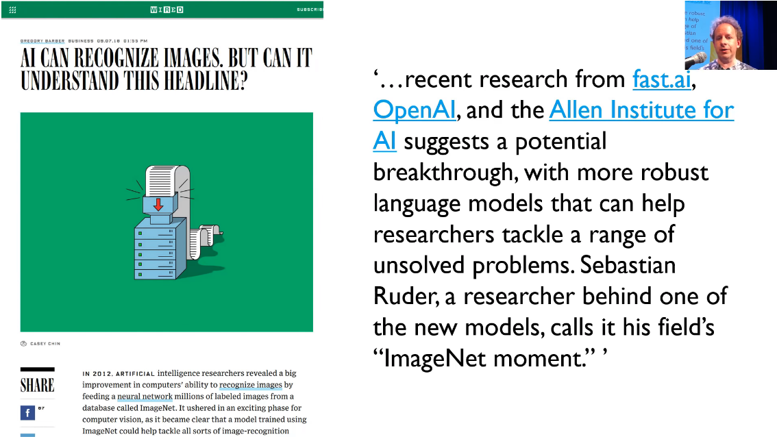
How far can you take it? All of the research that we do at fastai uses the library and an example of the research we did which was recently featured in Wired describes a new breakthrough in a natural language processing which people are calling the ImageNet moment which is basically we broke a new state-of-the-art result in text classification which OpenAI then built on top of our paper with more computing, more data to do different tasks to take it even further. This is an example of something we've done in the last 6 months in conjunction with my colleague Sebastian Ruder - an example of something that's being built in the fastai library and you are going to learn how to use this brand new model in three lessons time. You're actually going to get this exact result from this exact paper yourself.
[51:50]
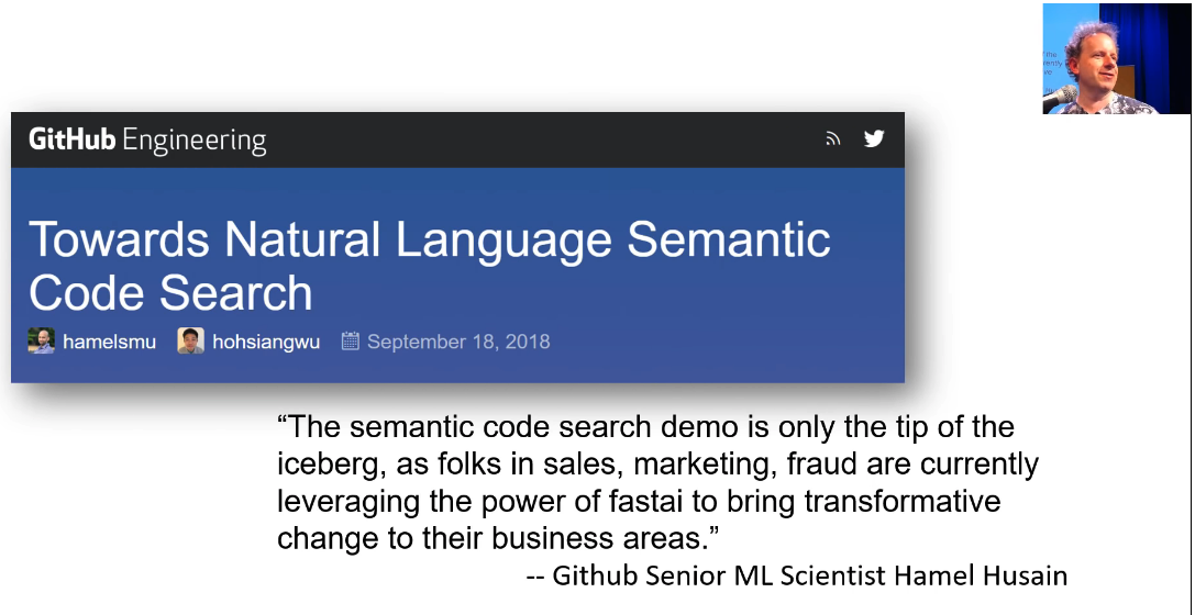
Another example, one of our alumni, Hamel Husain built a new system for natural language semantic code search, you can find it on Github where you can actually type in English sentences and find snippets of code that do the thing you asked for. Again, it's being built with the fastai library using the techniques you'll learn in the next seven weeks.
[52:27]
The best place to learn about these things and get involved in these things is on the forums where as well as categories for each part of the course and there is also a general category for deep learning where people talk about research papers applications.
Even though today, we are focusing on a small number of lines of code to a particular thing which is image classification and we are not learning much math or theory, over these seven weeks and then part two, we are going to go deeper and deeper.
Where can that take you? [53:05]
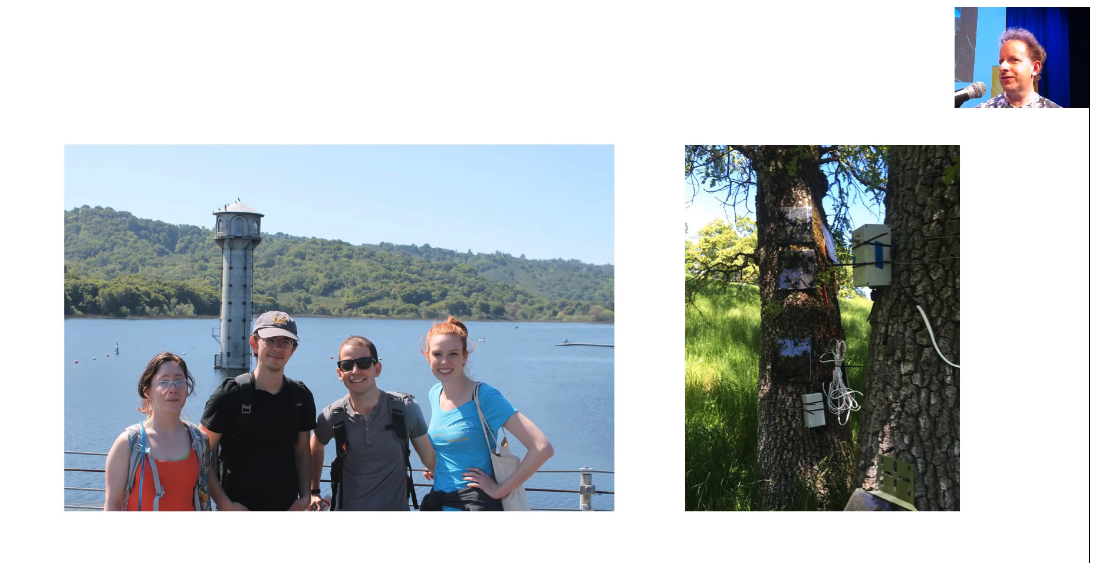
This is Sarah Hooker. She did our first course a couple of years ago. She started learning to code two years before she took our course. She started a nonprofit called Delta Analytics, they helped build this amazing system where they attached old mobile phones to trees in Kanyan rain forests and used it to listen for chainsaw noises, and then they used deep learning to figure out when there was a chainsaw being used and then they had a system setup to alert rangers to go out and stop illegal deforestation in the rainforests. That was something she was doing while she was in the course as part of her class projects.
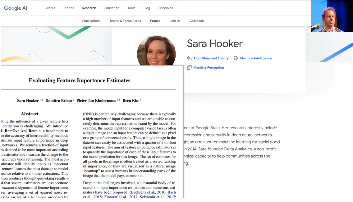
She is now a Google Brain researcher, publishing some papers, and now she is going to Africa to set up a Google Brain's first deep learning research center in Africa. She worked her arse off. She really really invested in this course. Not just doing all of the assignments but also going out and reading Ian Goodfellow's book, and doing lots of other things. It really shows where somebody who has no computer science or math background at all can be now one of the world's top deep learning researchers and doing very valuable work.
[54:49]
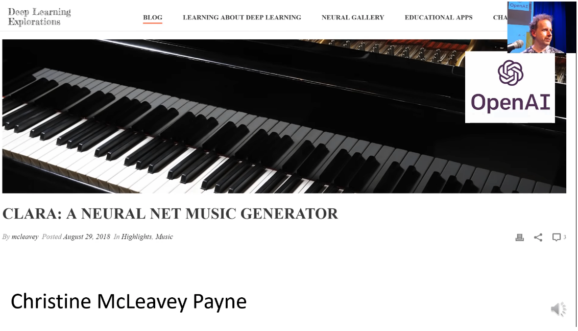
Another example from our most recent course, Christine Payne. She is now at OpenAI and you can find her post and actually listen to her music samples of something she built to automatically create chamber music compositions.
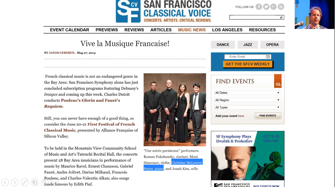
She is a classical pianist. Now I will say she is not your average classical pianist. She's a classical pianist who also has a master's in medical research in Stanford, and studied neuroscience, and was a high-performance computing expert at DE Shaw, Co-Valedictorian at Princeton. Anyway. Very annoying person, good at everything she does. But I think it's really cool to see how a domain expert of playing piano can go through the fastai course and come out the other end as OpenAI fellow.
Interestingly, one of our other alumni (Sanyam Bhutani) of the course recently interviewed her for a blog post series he is doing on top AI researchers and she said one of the most important pieces of advice she got was from me and she said the advice was:
Pick one project. Do it really well. Make it fantastic. 56:20
We're going to be talking a lot about you doing projects and making them fantastic during this course.
[56:36] Having said that, I don't really want you to go to AI or Google Brain. What I really want you to do is to go back to your workplace or your passion project and apply these skills there.
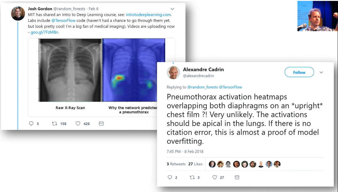
MIT released a deep learning course and they highlighted in their announcement this medical imaging example. One of our students Alex who is a radiologist said you guys just showed a model overfitting. I can tell because I am a radiologist and this is not what this would look like on a chest film. This is what it should look like and as a deep learning practitioner, this is how I know this is what happened in your model. So Alex is combining his knowledge of radiology and his knowledge of deep learning to assess MIT's model from just two images very accurately. So this is actually what I want most of you to be doing is to take your domain expertise and combine it with the deep learning practical aspects you'll learn in this course and bring them together like Alex is doing here. So a lot of radiologists have actually gone through this course now and have built journal clubs and American Council of Radiology practice groups. There's a data science institute at the ACR now and Alex is one of the people who is providing a lot of leadership in this area. And I would love you to do the same kind of thing that Alex is doing which is to really bring deep learning leadership into your industry and to your social impact project, whatever it is that you are trying to do.
[58:22]
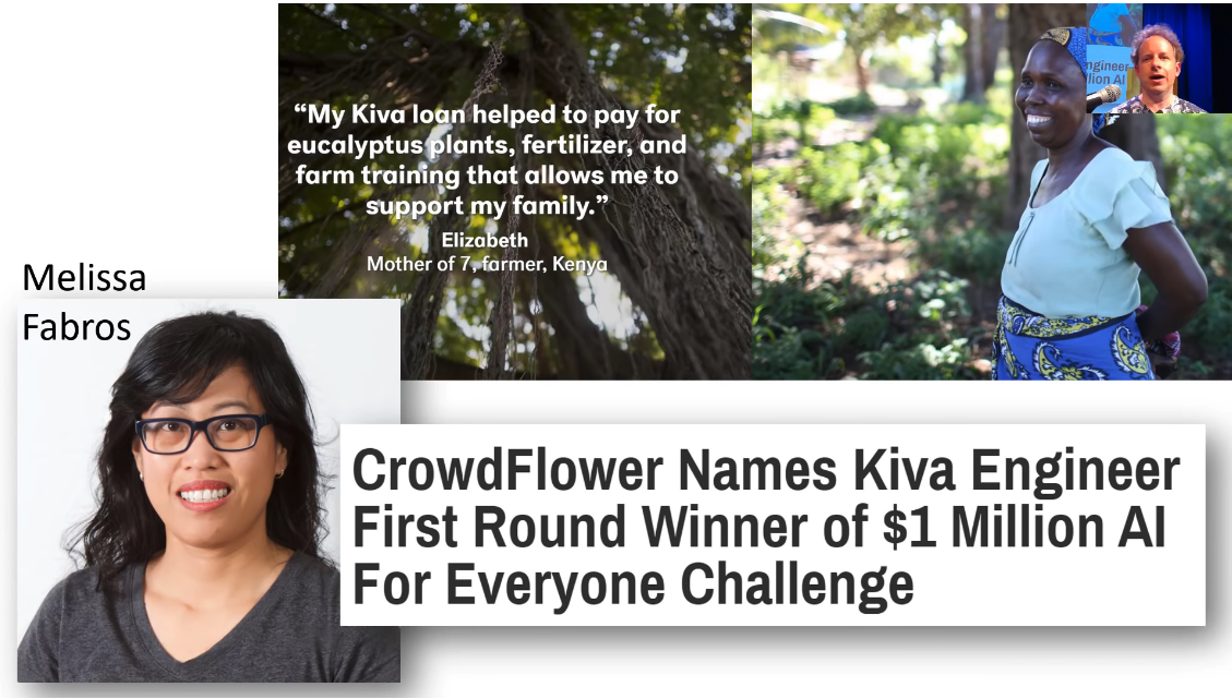
Another great example. This is Melissa Fabros who is a English literature PhD who studied gendered language in English literature or something and actually Rachel at the previous job taught her to code. Then she came to the fastai course. She helped Kiva, a micro lending a social impact organization, to build a system that can recognize faces. Why is that necessary? We're going to be talking a lot about this but because most AI researchers are white men, most computer vision software can only recognize white male faces effectively. In fast, I think it was IBM system was like 99.8% accurate on common white face men versus 65% accurate on dark skinned women. So it's like 30 or 40 times worse for black women versus white men. This is really important because for Kiva, black women perhaps are the most common user base for their micro lending platform. So Melissa after taking our course, again working her arse off, and being super intense in her study and her work won this $1,000,000 AI challenge for her work for Kiva.
[59:53]
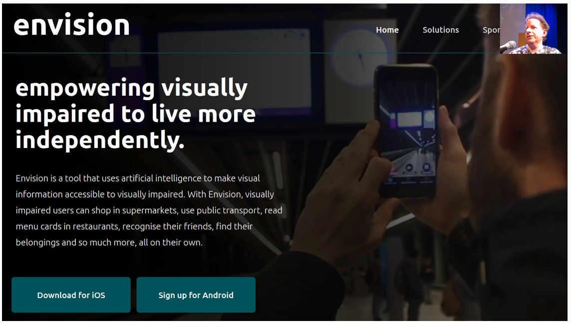
Karthik did our course and realized that the thing he wanted to do wasn't at his company. It was something else which is to help blind people to understand the world around them. So he started a new startup called envision. You can download the app and point your phone to things and it will tell you what it sees. I actually talked to a blind lady about these kinds of apps the other day and she confirmed to me this is a super useful thing for visually disabled users.
[1:00:24]
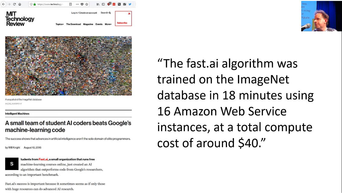
The level that you can get to, with the content that you're going to get over these seven weeks and with this software can get you right to the cutting edge in areas you might find surprising. I helped a team of some of our students and some collaborators on actually breaking the world record for how quickly you can train ImageNet. We used standard AWS cloud infrastructure, cost of $40 of compute to train this model using fastai library, the technique you learn in this course. So it can really take you a long way. So don't be put off by this what might seem pretty simple at first. We are going deeper and deeper.
[1:01:17]
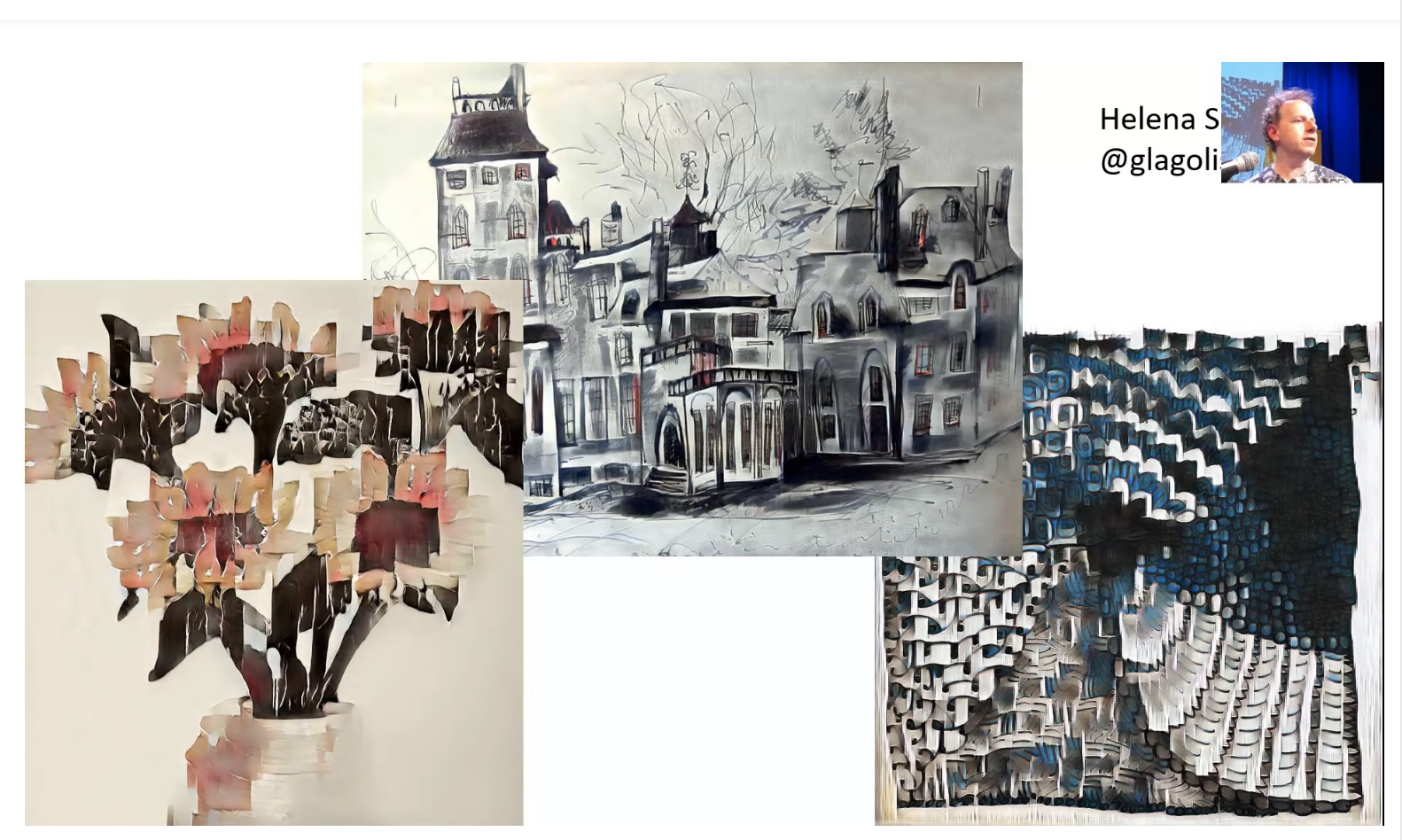
You can also use it for other kinds of passion project. Helena Sarin - you should definitely check out her Twitter account @glagolista. This art is basically a new style of art that she's developed which combines her painting and drawing with generative adversarial models to create these extraordinary results. I think this is super cool. She is not a professional artists, she is a professional software developer but she keeps on producing these beautiful results. When she started, her art had not really been shown or discussed anywhere, now there's recently been some quite high profile article describing how she is creating a new form of art.
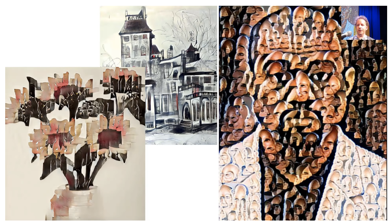
Equally important, Brad Kenstler who figured out how to make a picture of Kanye out of pictures of Patrick Stewart's head. Also something you will learn to do if you wish to. This particular type of what's called "style transfer" - it's a really interesting tweak that allowed him to do something that hadn't quite been done before. This particular picture helped him to get a job as a deep learning specialist at AWS.
[1:02:41]
Another alumni actually worked at Splunk as a software engineer and he designed an algorithm which basically turned Splunk to be fantastically good at identifying fraud and we'll talk more about it shortly.
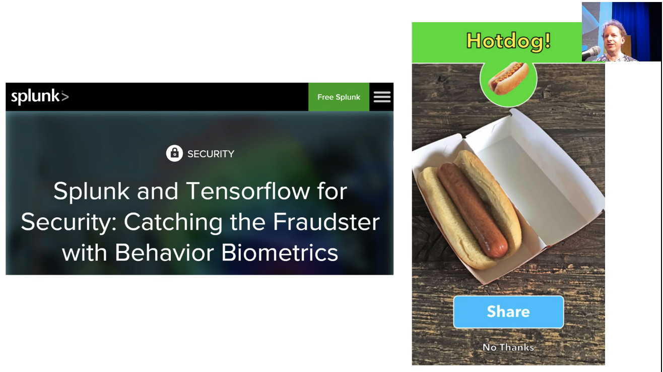
If you've seen Silicon Valley, the HBO series, the hotdog Not Hotdog app - that's actually a real app you can download and it was built by Tim Anglade as a fastai student project. So there's a lot of cool stuff that you can do. It was Emmy nominated. We only have one Emmy nominated fastai alumni at this stage, so please help change that.
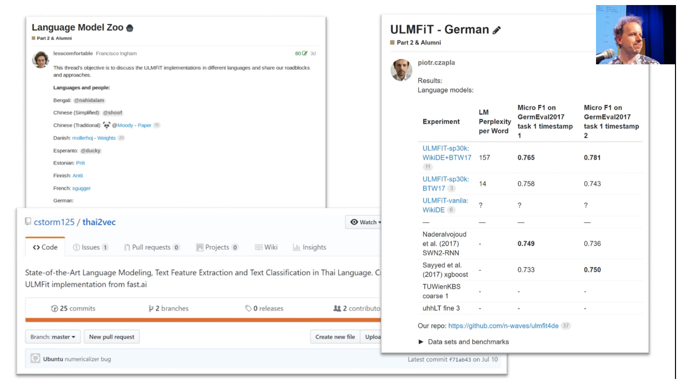 [1:03:30]
The other thing, the forum thread can turn into these really cool things. So Francisco was a really boring McKinsey consultant like me. So Francisco and I both have this shameful past that we were McKinsey consultants, but we left and we're okay now. He started this thread saying like this stuff we've just been learning about building NLP in different languages, let's try and do lots of different languages, and he started this thing called the language model zoo and out of that, there's now been an academic competition was won in Polish that led to an academic paper, Thai state of the art, German state of the art, basically as students have been coming up with new state of the art results across lots of different languages and this all is entirely done by students working together through the forum.
So please get on the forum. But don't be intimidated because everybody you see on the forum, the vast majority of posting post all the darn time. They've been doing this a lot and they do it a lot of the time. So at first, it can feel intimidating because it can feel like you're the only new person there. But you're not. You're all new people, so when you just get out there and say like "okay all you people getting these state of the art results in German language modeling, I can't start my server, I try to click the notebook and I get an error, what do I do?" People will help you. Just make sure you provide all the information (how to ask for help).
Or if you've got something to add! If people are talking about crop yield analysis and you're a farmer and you think oh I've got something to add, please mention it even if you are not sure it's exactly relevant. It's fine. Just get involved. Because remember, everybody else in the forum started out also intimidated. We all start out not knowing things. So just get out there and try it!
[1:05:59] Question❓: Why are we using ResNet as opposed to Inception?
There are lots of architectures to choose from and it would be fair to say there isn't one best one but if you look at things like the Stanford DAWNBench benchmark of ImageNet classification, you'll see in first place, second place, third place, and fourth place all use ResNet. ResNet is good enough, so it's fine. 😆😆😆
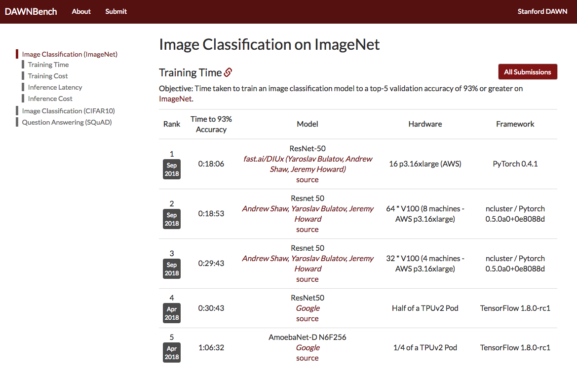
The main reason you might want a different architecture is if you want to do edge computing, so if you want to create a model that's going to sit on somebody's mobile phone. Having said that, even there, most of the time, I reckon the best way to get a model onto somebody's mobile phone is to run it on your server and then have your mobile phone app talk to it. It really makes life a lot easier and you get a lot more flexibility. But if you really do need to run something on a low powered device, then there are special architectures for that. So the particular question was about Inception. That's a particular another architecture which tends to be pretty memory intensive but it's okay. It's not terribly resilient. One of the things we try to show you is stuff which just tends to always work even if you don't quite tune everything perfectly. So ResNet tends to work pretty well across a wide range of different kind of details around choices that you might make. So I think it's pretty good.
[1:07:58]
We've got this trained model and what's actually happened as we'll learn is it's basically creating a set of weights. If you've ever done anything like a linear regression or logistic regression, you'll be familiar with coefficients. We basically found some coefficients and parameters that work pretty well and it took us a minute and 56 seconds. So if we want to start doing some more playing around and come back later, we probably should save those weights. You can just go learn.save and give it a name. It's going to put it in a model subdirectory in the same place the data came from, so if you save different models or different DataBunches from different datasets, they'll all be kept separate. So don't worry about it.
learn.save('stage-1')
Results [1:08:54]
To see what comes out, we could use this class for class interpretation. We are going to use this factory method from learner, so we pass in a learn object. Remember a learn object knows two things:
- What's your data
- What is your model. Now it's not just an architecture, it's actually a trained model
That's all the information we need to interpret that model.
interp = ClassificationInterpretation.from_learner(learn)
One of the things, perhaps the most useful things to do is called plot_top_losses. We are going to be learning a lot about this idea of loss functions shortly but in short, a loss function is something that tells you how good was your prediction. Specifically that means if you predicted one class of cat with great confidence, but actually you were wrong, then that's going to have a high loss because you were very confident about the wrong answer. So that's what it basically means to have high loss. By plotting the top losses, we are going to find out what were the things that we were the most wrong on, or the most confident about what we got wrong.
interp.plot_top_losses(9, figsize=(15,11))
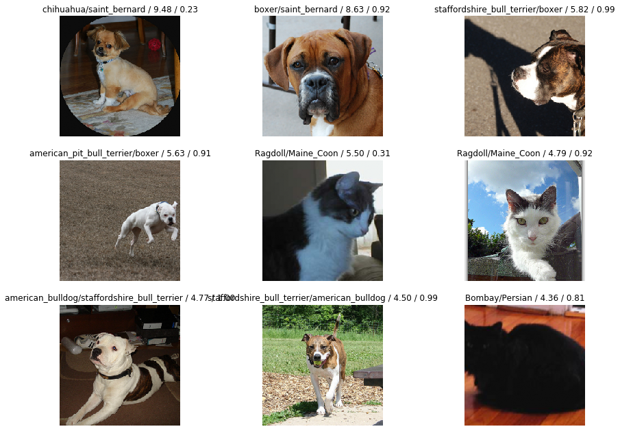
It prints out four things. What do they mean? Perhaps we should look at the document.
We have already seen help, and help just prints out a quick little summary. But if you want to really see how to do something use doc.
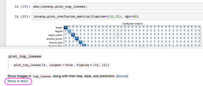
doc tells you the same information as help but it has this very important thing which is Show in docs. When you click on it, it pops up the documentation for that method or class or function or whatever:
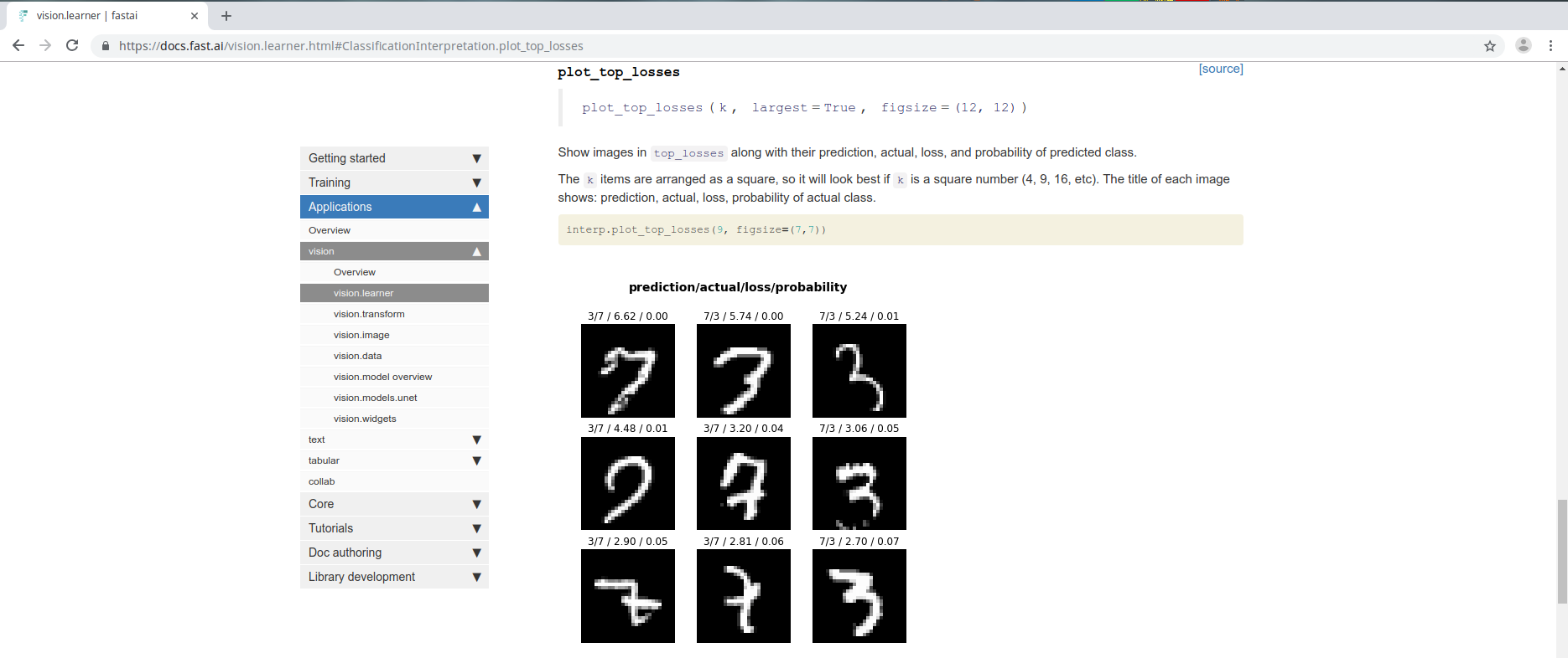
It starts out by showing us the same information about what are the parameters it takes a long with the docstring. But then tells you more information:
The title of each image shows: prediction, actual, loss, probability of actual class.
The documentation always has working code. This is your friend when you're trying to figure out how to use these things. The other thing I'll mention is if you're somewhat experienced Python programmer, you'll find the source code of fastai really easy to read. We are trying to write everything in just a small number (much less than half a screen) of code. If you click on [source] you can jump straight to the source code.

Here is plot_top_loss, and this is also a great way to find out how to use the fastai library. Because nearly every line of code here, is calling stuff in the fastai library. So don't be afraid to look at the source code.
[1:12:48]
So that's how we can look at top losses and these are perhaps the most important image classification interpretation tools that we have because it lets us see what we are getting wrong.
📢 fastai had a bug when this code was run - your numbers will look different to this!
In this case, if you are a dog and cat expert, you'll realize that the things that's getting wrong are breeds that are actually very difficult to tell apart and you'd be able to look at these and say "oh I can see why they've got this one wrong". So this is a really useful tool.
Confusion matrix [1:13:21]
Another useful tool, kind of, is to use something called a confusion matrix which basically shows you for every actual type of dog or cat, how many times was it predicted to be that dog or cat. But unfortunately, in this case, because it's so accurate, this diagonal basically says how it's pretty much right all the time.
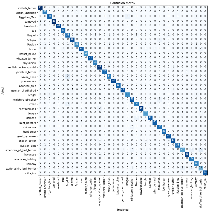
And you can see there is slightly darker ones like a five here, it's really hard to read exactly what their combination is. So what I suggest you use is instead of, if you've got lots of classes, don't use confusion matrix, but this is my favorite named function in fastai and I'm very proud of this - you can call "most confused".
Most confused [1:13:52]
interp.most_confused(min_val=2)

# -----------------------------------------------------------------------------
# Output
# -----------------------------------------------------------------------------
[('american_pit_bull_terrier', 'staffordshire_bull_terrier', 6),
 ('Birman', 'Ragdoll', 5),
 ('english_setter', 'english_cocker_spaniel', 4),
 ('staffordshire_bull_terrier', 'american_pit_bull_terrier', 4),
 ('boxer', 'american_bulldog', 4),
 ('Ragdoll', 'Birman', 3),
 ('miniature_pinscher', 'chihuahua', 3),
 ('Siamese', 'Birman', 3)]
most_confused will simply grab out of the confusion matrix the particular combinations of predicted and actual that got wrong the most often. So this case, ('american_pit_bull_terrier', 'staffordshire_bull_terrier', 6):
- Actual
'american_pit_bull_terrier' - Prediction
'staffordshire_bull_terrier' - This particular combination happened 6 times.
So this is a very useful thing because you can look and say "with my domain expertise, does it make sense" that would be something that was confused about?
Unfreezing, fine-tuning, and learning rates [1:14:38]
Let's make our model better. How do we make it better? By using fine-tuning. So far we fitted 4 epochs and it ran pretty quickly. The reason it ran pretty quickly is that there was a little trick we used. These convolutional networks, they have many layers. We'll learn a lot about exactly what layers are, but for now, just know it goes through a lot of computations. What we did was we added a few extra layers to the end and we only trained those. We basically left most of the model exactly as it was, so that's really fast. If we are trying to build a model at something that's similar to the original pre-trained model (in this case, similar to the ImageNet data), that works pretty well.
But what we really want to do is to go back and train the whole model. This is why we pretty much always use this two stage process. By default, when we call fit or fit_one_cycle on a ConvLearner, it'll just fine-tune these few extra layers added to the end and it will run very fast. It will basically never overfit but to really get it good, you have to call unfreeze. unfreeze is the thing that says please train the whole model. Then I can call fit_one_cycle again.
learn.unfreeze()
learn.fit_one_cycle(1)

# -----------------------------------------------------------------------------
# Output
# -----------------------------------------------------------------------------
Total time: 00:20
epoch  train_loss  valid_loss  error_rate
1      1.045145    0.505527    0.159681    (00:20)
Uh-oh. The error got much worse. Why? In order to understand why, we are actually going to have to learn more about exactly what's going on behind the scenes. So let's start out by trying to get an intuitive understanding of what's going on behind the scenes. We are going to do it by looking at pictures.
[1:16:28]
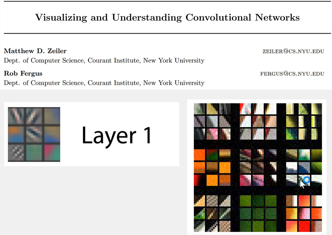
These pictures come from a fantastic paper by Matt Zeiler who nowadays is a CEO of Clarify which is a very successful computer vision startup and his supervisor for his PhD Rob Fergus. They wrote a paper showing how you can visualize the layers of a convolutional neural network. A convolutional neural network, which we will learn mathematically about what the layers are shortly, but the basic idea is that your red, green, and blue pixel values that are numbers from nought to 255 go into the simple computation (i.e. the first layer) and something comes out of that, and then the result of that goes into a second layer, and the result of that goes into the third layer and so forth. There can be up to a thousand layers of neural network. ResNet34 has 34 layers, and ResNet50 has 50 layers, but let's look at layer one. There's this very simple computation which is a convolution if you know what they are. What comes out of this first layer? Well, we can actually visualize these specific coefficients, the specific parameters by drawing them as a picture. There's actually a few dozen of them in the first layer, so we don't draw all of them. Let's just look at 9 at random.
[1:17:45]
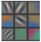
Here are nine examples of the actual coefficients from the first layer. So these operate on groups of pixels that are next to each other. So this first one basically finds groups of pixels that have a little diagonal line, the second one finds diagonal line in the other direction, the third one finds gradients that go from yellow to blue, and so forth. They are very simple little filters. That's layer one of ImageNet pre-trained convolutional neural net.
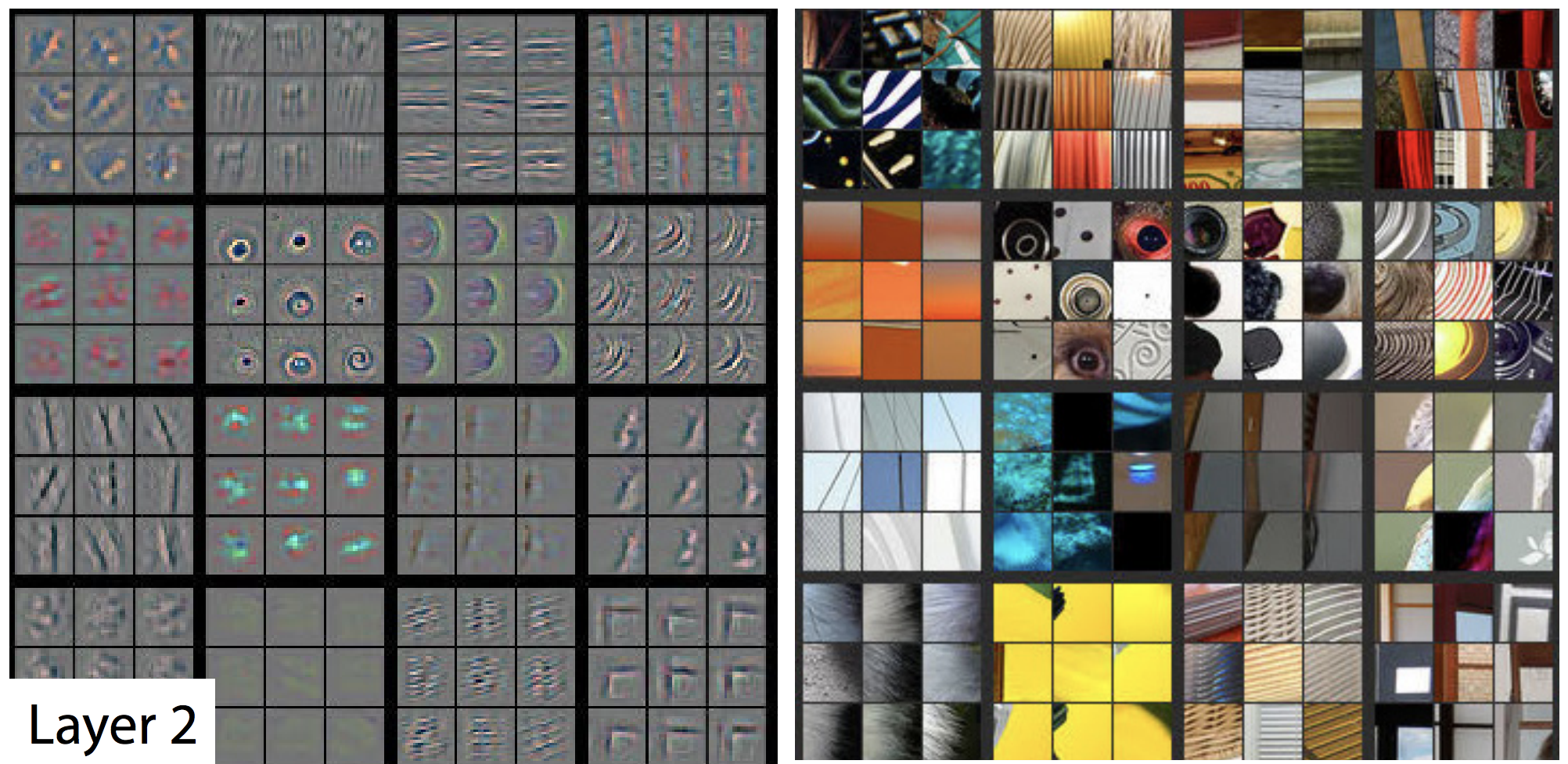
Layer 2 takes the results of those filters and does a second layer of computation. The bottom right are nine examples of a way of visualizing one of the second layer features. AS you can see, it basically learned to create something that looks for top left corners. There are ones that learned to find right-hand curves, and little circles, etc. In layer one, we have things that can find just one line, and in layer 2, we can find things that have two lines joined up or one line repeated. If you then look over to the right, these nine show you nine examples of actual bits of the actual photos that activated this filter a lot. So in other words, the filter on the bottom right was good at finding these window corners etc.
So this is the kind of stuff you've got to get a really good intuitive understanding for. The start of my neural net is going to find very simple gradients and lines, the second layer can find very simple shapes, the third layer can find combination of those.
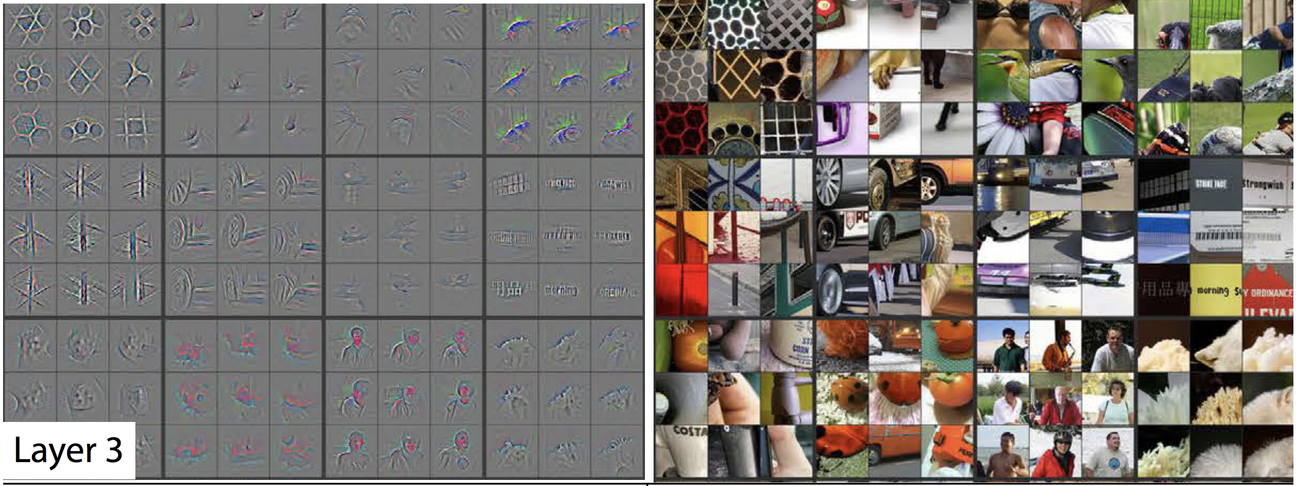
Now we can find repeating pattern of two dimensional objects or we can find things that joins together, or bits of text (although sometimes windows) - so it seems to find repeated horizontal patterns. There are also ones that seem to find edges of fluffy or flowery things or geometric patterns. So layer 3 was able to take all the stuff from layer 2 and combine them together.
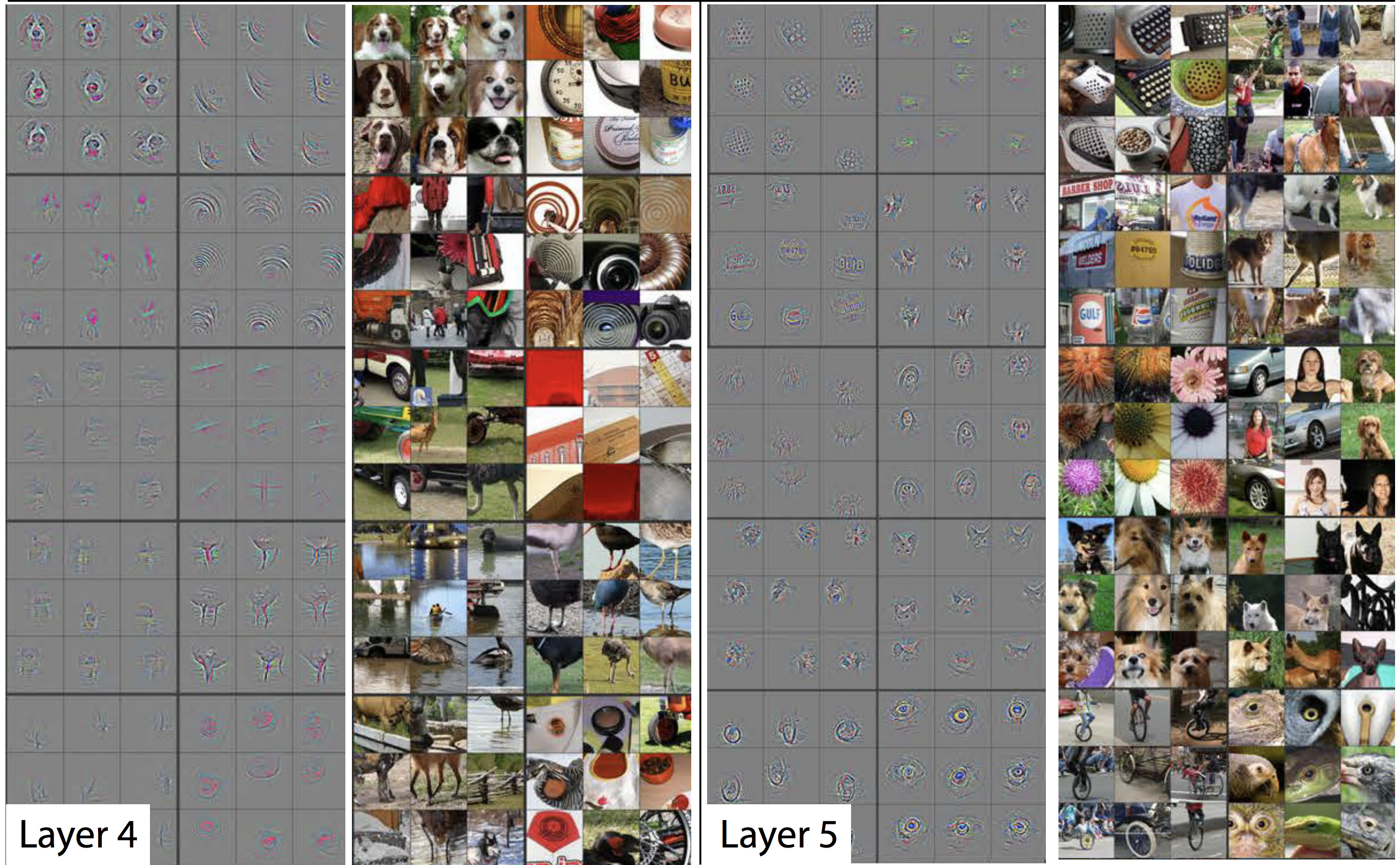
Layer 4 can take all the stuff from layer 3 and combine them together. By layer 4, we got something that can find dog faces or bird legs.
By layer 5, we've got something that can find the eyeballs of bird and lizards, or faces of particular breeds of dogs and so forth. So you can see how by the time you get to layer 34, you can find specific dog breeds and cat breeds. This is kind of how it works.
So when we first trained (i.e. fine-tuned) the pre-trained model, we kept all of these layers that you've seen so far and we just trained a few more layers on top of all of those sophisticated features that are already being created. So now we are going back and saying "let's change all of these". We will start with where they are, but let's see if we can make them better.
Now, it seems very unlikely that we can make layer 1 features better. It's very unlikely that the definition of a diagonal line is going to be different when we look at dog and cat breeds versus the ImageNet data that this was originally trained on. So we don't really want to change the layer 1 very much if at all. Or else, the last layers, like types of dog face seems very likely that we do want to change that. So you want this intuition, this understanding that the different layers of a neural network represents different level of semantic complexity.
[1:22:06]
This is why our attempt to fine-tune this model didn't work because by default, it trains all the layers at the same speed which is to say it will update those things representing diagonal lines and gradients just as much as it tries to update the things that represent the exact specifics of what an eyeball looks like, so we have to change that.
To change it, we first of all need to go back to where we were before. We just broke this model, much worse than it started out. So if we just go:
learn.load('stage-1')
This brings back the model that we saved earlier. So let's load that back up and now our models back to where it was before we killed it.
Learning rate finder [1:22:58]
Let's run learning rate finder. We are learning about what that is next week, but for now, just know this is the thing that figures out what is the fastest I can train this neural network at without making it zip off the rails and get blown apart.
learn.lr_find()
learn.recorder.plot()
This will plot the result of our LR finder and what this basically shows you is this key parameter called a learning rate. The learning rate basically says how quickly am I updating the parameters in my model. The x-axis one here shows me what happens as I increase the learning rate. The y axis show what the loss is. So you can see, once the learning rate gets passed 10^-4, my loss gets worse. It actually so happens, in fact I can check this if I press shift+tab here, my learning defaults to 0.003. So you can see why our loss got worse. Because we are trying to fine-tune things now, we can't use such a high learning rate. So based on the learning rate finder, I tried to pick something well before it started getting worse. So I decided to pick 1e-6. But there's no point training all the layers at that rate, because we know that the later layers worked just fine before when we were training much more quickly. So what we can actually do is we can pass a range of learning rates to learn.fit_one_cycle. And we do it like this:
learn.unfreeze()
learn.fit_one_cycle(2, max_lr=slice(1e-6,1e-4))

# -----------------------------------------------------------------------------
# Output
# -----------------------------------------------------------------------------
Total time: 00:41
epoch  train_loss  valid_loss  error_rate
1      0.226494    0.173675    0.057219    (00:20)
2      0.197376    0.170252    0.053227    (00:20)
You use this keyword in Python called slice and that can take a start value and a stop value and basically what this says is train the very first layers at a learning rate of 1e-6, and the very last layers at a rate of 1e-4, and distribute all the other layers across that (i.e. between those two values equally).
How to pick learning rates after unfreezing [1:25:23]
A good rule of thumb is after you unfreeze (i.e. train the whole thing), pass a max learning rate parameter, pass it a slice, make the second part of that slice about 10 times smaller than your first stage. Our first stage defaulted to about 1e-3 so it's about 1e-4. And the first part of the slice should be a value from your learning rate finder which is well before things started getting worse. So you can see things are starting to get worse maybe about here:

So I picked something that's at least 10 times smaller than that.
If I do that, then the error rate gets a bit better. So I would perhaps say for most people most of the time, these two stages are enough to get pretty much a world-class model. You won't win a Kaggle competition, particularly because now a lot of fastai alumni are competing on Kaggle and this is the first thing that they do. But in practice, you'll get something that's about as good in practice as the vast majority of practitioners can do.
ResNet50 [1:26:55]
We can improve it by using more layers and we will do this next week but by basically doing a ResNet50 instead of ResNet34. And you can try running this during the week if you want to. You'll see it's exactly the same as before, but I'm using ResNet50.
data = ImageDataBunch.from_name_re(path_img, fnames, pat, ds_tfms=get_transforms(), size=320, bs=bs//2)
data.normalize(imagenet_stats)
learn = ConvLearner(data, models.resnet50, metrics=error_rate)
What you'll find is it's very likely if you try to do this, you will get an error and the error will be your GPU has ran out of memory. The reason for that is that ResNet50 is bigger than ResNet34, and therefore, it has more parameters and use more of your graphics card memory, just totally separate to your normal computer RAM, this is GPU RAM. If you're using the default Salamander, AWS, and so forth, then you'll be having a 16G of GPU memory. The card I use most of the time has 11G GPU memory, the cheaper ones have 8G. That's kind of the main range you tend to get. If yours have less than 8G of GPU memory, it's going to be frustrating for you.
It's very likely that if you try to run this, you'll get an out of memory error and that's because it's just trying to do too much - too many parameter updates for the amount of RAM you have. That's easily fixed. ImageDataBunch constructor has a parameter at the end bs - a batch size. This basically says how many images do you train at one time. If you run out of memory, just make it smaller.
It's fine to use a smaller batch size. It might take a little bit longer. That's all. So that's just one number you'll need to try during the week.
learn.fit_one_cycle(8, max_lr=slice(1e-3))

# -----------------------------------------------------------------------------
# Output
# -----------------------------------------------------------------------------
Total time: 07:08
epoch  train_loss  valid_loss  error_rate
1      0.926640    0.320040    0.076555    (00:52)
2      0.394781    0.205191    0.063568    (00:52)
3      0.307754    0.203281    0.069036    (00:53)
4      0.244182    0.160488    0.054682    (00:53)
5      0.185785    0.153520    0.049214    (00:53)
6      0.157732    0.149660    0.047163    (00:53)
7      0.107212    0.136898    0.043062    (00:53)
8      0.097324    0.136638    0.042379    (00:54)
Again, we fit it for a while and we get down to 4.2% error rate. So this is pretty extraordinary. I was pretty surprised because when we first did in the first course, this cats vs. dogs, we were getting somewhere around 3% error for something where you've got a 50% chance of being right and the two things look totally different. So the fact that we can get 4.2% error for such a fine grain thing, it's quite extraordinary.
Interpreting the results again [1:29:41]
interp = ClassificationInterpretation.from_learner(learn)
interp.most_confused(min_val=2)

# -----------------------------------------------------------------------------
# Output
# -----------------------------------------------------------------------------
[('Ragdoll', 'Birman', 7),
 ('american_pit_bull_terrier', 'staffordshire_bull_terrier', 6),
 ('Egyptian_Mau', 'Bengal', 6),
 ('Maine_Coon', 'Bengal', 3),
 ('staffordshire_bull_terrier', 'american_pit_bull_terrier', 3)]
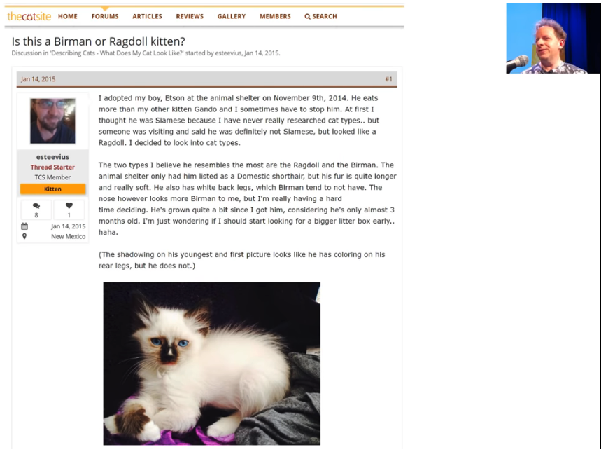
You can call the most_confused here and you can see the kinds of things that it's getting wrong. Depending on when you run it, you're going to get slightly different numbers, but you'll get roughly the same kind of things. So quite often, I find the Ragdoll and Birman are things that it gets confused. I actually have never heard of either of those things, so I actually looked them up and found a page on the cat site called "Is this a Birman or Ragdoll kitten?" and there was a long thread of cat experts arguing intensely about which it is. So I feel fine that my computer had problems. 😆😆😆
I found something similar, I think it was this pitbull versus staffordshire bull terrier, apparently the main difference is the particular kennel club guidelines as to how they are assessed. But some people think that one of them might have a slightly redder nose. So this is the kind of stuff where actually even if you're not a domain expert, it helps you become one. Because I now know more about which kinds of pet breeds are hard to identify than I used to. So model interpretation works both ways.
Homework [1:30:58]
So what I want you to do this week is to run this notebook, make sure you can get through it, but then I really want you to do is to get your own image dataset and actually Francisco who is now helping to TA the course is putting together a guide that will show you how to download data from Google Images so you can create your own dataset to play with. But before I do, I want to show you how to create labels in lots of different ways because your dataset where you get it from won't necessarily be that kind of regex based approach. It could be in lots of different formats. So to show you how to do this, I'm going to use the MNIST sample. MNIST is a picture of hand drawn numbers - just because I want to show you different ways of creating these datasets.
path = untar_data(URLs.MNIST_SAMPLE); path
path.ls()

# -----------------------------------------------------------------------------
# Output
# -----------------------------------------------------------------------------
['train', 'valid', 'labels.csv', 'models']
You see there are a training set and the validation set already. So basically the people that put together this dataset have already decided what they want you to use as a validation set.
Possibility 1: Labels are folder names
(path/'train').ls()

# -----------------------------------------------------------------------------
# Output
# -----------------------------------------------------------------------------
['3', '7']
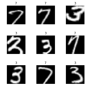
There are a folder called 3 and a folder called 7. Now this is really common way to give people labels. Basically it says everything that's a three, I put in a folder called three. Everything that's a seven, I'll put in a folder called seven. This is often called an "ImageNet style dataset" because this is how ImageNet is distributed. So if you have something in this format where the labels are just whatever the folders are called, you can say from_folder.
tfms = get_transforms(do_flip=False)
data = ImageDataBunch.from_folder(path, ds_tfms=tfms, size=26)
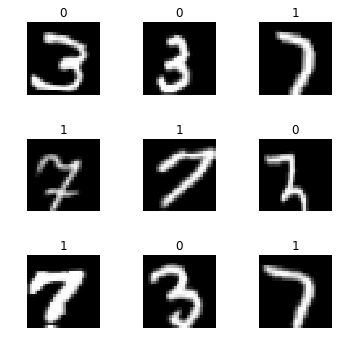
This will create an ImageDataBunch for you and as you can see it created the labels:
data.show_batch(rows=3, figsize=(5,5))
Possibility 2: CSV file [1:33:17]
Another possibility, and for this MNIST sample, I've got both, it might come with a CSV file that would look something like this.
df = pd.read_csv(path/'labels.csv')
df.head()
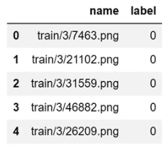
For each file name, what's its label. In this case, labels are not three or seven, they are 0 or 1 which basically is it a 7 or not. So that's another possibility. If this is how your labels are, you can use from_csv:
data = ImageDataBunch.from_csv(path, ds_tfms=tfms, size=28)
And if it is called labels.csv, you don't even have to pass in a file name. If it's called something else, then you can pass in the csv_labels
data.show_batch(rows=3, figsize=(5,5))
data.classes

# -----------------------------------------------------------------------------
# Output
# -----------------------------------------------------------------------------
[0, 1]
Possibility 3: Using regular expression
fn_paths = [path/name for name in df['name']]; fn_paths[:2]

# -----------------------------------------------------------------------------
# Output
# -----------------------------------------------------------------------------
[PosixPath('/home/jhoward/.fastai/data/mnist_sample/train/3/7463.png'),
 PosixPath('/home/jhoward/.fastai/data/mnist_sample/train/3/21102.png')]
This is the same thing, these are the folders. But I could actually grab the label by using a regular expression. We've already seen this approach:
pat = r"/(\d)/\d+\.png$"
data = ImageDataBunch.from_name_re(path, fn_paths, pat=pat, ds_tfms=tfms, size=24)
data.classes

# -----------------------------------------------------------------------------
# Output
# -----------------------------------------------------------------------------
['3', '7']
Possibility 4: Something more complex [1:34:21]
You can create an arbitrary function that extracts a label from the file name or path. In that case, you would say from_name_func:
data = ImageDataBunch.from_name_func(path, fn_paths, ds_tfms=tfms, size=24,
        label_func = lambda x: '3' if '/3/' in str(x) else '7')
data.classes
Possibility 5: You need something even more flexible
If you need something even more flexible than that, you're going to write some code to create an array of labels. So in that case, you can just use from_lists and pass in the array.
labels = [('3' if '/3/' in str(x) else '7') for x in fn_paths]
labels[:5]
data = ImageDataBunch.from_lists(path, fn_paths, labels=labels, ds_tfms=tfms, size=24)
data.classes
So you can see there's lots of different ways of creating labels. So during the week, try this out.
Now you might be wondering how would you know to do all these things? Where am I going to find this kind of information? So I'll show you something incredibly cool. You know how to get documentation:
doc(ImageDataBunch.from_name_re)
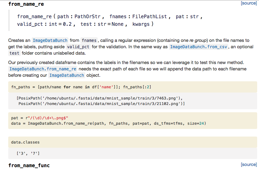
Here's the thing, every single line of code I just showed you, I took it this morning and I copied and pasted it from the documentation. So you can see here the exact code that I just used. So the documentation for fastai doesn't just tell you what to do, but step to step how to do it. And here is perhaps the coolest bit. If you go to fastai/fastai_docs and click on docs/src.
All of our documentation is actually just Jupyter Notebooks. You can git clone this repo and if you run it, you can actually run every single line of the documentation yourself.
This is the kind of the ultimate example to me of experimenting. Anything that you read about in the documentation, nearly everything in the documentation has actual working examples in it with actual datasets that are already sitting in there in the repo for you. So you can actually try every single function in your browser, try seeing what goes in and try seeing what comes out.
[1:37:27] Question❓: Will the library use multi GPUs in parallel by default?
The library will use multiple CPUs by default but just one GPU by default. We probably won't be looking at multi GPU until part 2. It's easy to do and you'll find it on the forum, but most people won't be needing to use that now.
Question❓: Can the library use 3D data such as MRI or CAT scan?
Yes, it can. And there is actually a forum thread about that already. Although that's not as developed as 2D yet but maybe by the time the MOOC is out, it will be.
Splunk Anti-Fraud Software [1:38:10]
Before I wrap up, I'll just show you an example of the kind of interesting stuff that you can do by doing this kind of exercise.
Remember earlier I mentioned that one of our alumni who works at Splunk which is a NASDAQ listed big successful company created this new anti-fraud software. This is actually how he created it as part of a fastai part 1 class project:
He took the telemetry of users who had Splunk analytics installed and watched their mouse movements and he created pictures of the mouse movements. He converted speed into color and right and left clicks into splotches. He then took the exact code that we saw with an earlier version of the software and trained a CNN in exactly the same way we saw and used that to train his fraud model. So he took something which is not obviously a picture and he turned it into a picture and got these fantastically good results for a piece of fraud analysis software.
So it pays to think creatively. So if you are wanting to study sounds, a lot of people that study sounds do it by actually creating a spectrogram image and then sticking that into a ConvNet. So there's a lot of cool stuff you can do with this.
So during the week, get your GPU going, try and use your first notebook, make sure that you can use lesson 1 and work through it. Then see if you can repeat the process on your own dataset. Get on the forum and tell us any little success you had. Any constraints you hit, try it for an hour or two but if you get stuck, please ask. If you are able to successfully build a model with a new dataset, let us know! I will see you next week.
⚠️⚠️⚠️Don't forget to shutdown your GPU instance so that you don't keep getting charged!⚠️⚠️⚠️